Manual: 2.6. Data Requirements

Any analysis of data relies on the quality of the data provided. First and foremost, we assume that all important aspects of the process or equipment are included in the dataset. If important data is missing, then modeling may not work as well as it would if this data were included. On the other hand, it is not good to overload a model with a large number of unimportant measurements. The most important action for modeling is a sensible selection of tags to be included in the model. For an industrial plant with a complex control system, we can usually say that less than 10% of all available measurements are actually important for modeling the process.

However, in case of doubt, we recommend to include the measurement rather than exclude it. The reason for this is the same as in human learning. If you have irrelevant information, this is time-consuming and perhaps annoying but it will not prevent you from reaching understanding. However, if you lack important information, this may prevent you from achieving actual understanding. So it is best to err on the side of inclusion.

Most data historians have the policy of recording a new value for a tag only if it differs from the last recorded value by at least a certain amount. This amount is usually called the compression factor. This means that some measurements are recorded frequently and others very seldom. For mere recording this is a huge space saving mechanism.

For analysis and machine learning, we have to align the data however. For each time stamp, we must know the value of every tag at that time stamp. Most machine learning methods also require the time difference between successive time stamps to be the same.

In order to get from the usual historian policy to this aligned data table, we use the general rule that the value of a tag stays the same until we get a new one. A time-series may thus turn into something looking like a staircase. In most cases this data alignment leads to a growth in total data volume as there will be a number of duplicate values. This cannot be avoided however.

For this reason, we must choose a sensible data cadence. That is to say, the time difference between successive time stamps in this table must not be too small for reasons of data volume but also not too large so as to make the process dynamics invisible. The cadence must be chosen with care based on knowledge of the inherent time scale of the process that one wishes to model.

A dataset must have a beginning and an end. For training an IHM model, we must select the training data time period with care as we want to show a period of healthy behavior for the equipment in question. If we believe that external conditions, e.g. the seasons, matter for an accurate depiction of the process, then we need some data for these different conditions. For accurately modeling health on equipment, we usually find that a training time period of three to six weeks is sufficient. These weeks need not be consecutive. If we believe that seasons are important, we choose one week each in spring, summer, fall and winter. For optimization modeling e recommend a full year in order to include seasonal variations.

In the time periods used for training, we may have temporary conditions that should not be trained. If, for example, the equipment is turned off each night, we would not want to train the model during the hours that the equipment is not operating at all. For this reason, the software offers exclusion conditions based on the values of certain measurements. One might say for example that all data points where the rotation rate of the turbine is less than 500rpm must be excluded from modeling. The tags needed to make such judgments must be included in the dataset.

After these choices are made, the tags must be made known to the modeling system by providing some basic information about them. Apart from administrative information such as their names and units, we must know a few more facts. As measurement errors do occur in practice, we must know the range of measurements that are allowed so that a very low or very high measurement can be identified as an outlier and excluded. We need to know the measurement uncertainty so that we can compute the uncertainty in the result of the analysis; for more information about this, please see the section on mathematical background. For IHM, we need to know which of the measurements are to receive dynamic limits and are thus to be alarmed. In practice, most of the measurements in the model will not be alarmed but only used to provide context and information for those measurements that should receive alarms. For APO we must know which tags can be controlled directly by the operator and which cannot be controlled at all.

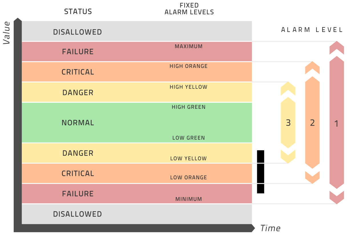
Optionally, you may specify up to three static alarm ranges for each measurement. This is provided so that IHM supports traditional condition monitoring in addition to its dynamic limit approach. This analysis and alarming is separate from the modeling analysis and thus totally optional. These ranges are best explained in the diagram below.

In summary, these are the initial choices to be made in relation to your dataset:

1. Which tags are to be included?
2. What data cadence is to be used?
3. What time period will the dataset have?
4. What are the time periods to be used for training?
5. What exclusion conditions should be applied?
6. For each tag …
   1. What is the allowed range of values?
   2. What is the tag uncertainty?
   3. Is this tag to be modeled and alarmed?
   4. Can this tag be directly controlled by the operator?
   5. Optionally, what are the static alarm ranges for yellow, orange and red alarms?