Manual PDF Export
1. Management
Congratulations on your decision to implement advanced analytics in your plant!
In order to get the most out of the experience of using analytics, we suggest that you take a little time to think about the managerial process of integrating this solution into your existing organization. Using a new capability is much more complex than installing a new software package.
In your planning, please consider such topics as
- The software installation will need IT experts to install the programs and also to setup the network permissions.
- Engineering experts will select the data to be used for modeling.
- Process experts will study the model, fine tune it, and decide its fitness for use.
- The end users of the software will need to be trained on how to use it.
- Management will need to decide on the usage policy.
- Action plans need to be established by change management in order to get practical use from the results of analytics.
- Feedback on the benefits earned and lessons learned will need to be communicated within your organization.
- Communication with algorithmica takes place when it appears that the model or the software needs to be adjusted or customized.
We therefore encourage you to think about this as a project management task in which there are stakeholders, a leadership team, a project manager and team members. We will not go into detail on the topic of project management in this manual but assume that your organization has that competency already.
The introduction of an analytics program will cause changes to the work environment for a number of people. Getting them used to the new way of working and integrating the technology into the work flow will be an adjustment. Some change management will need to occur for this to take hold in the organization.
1.1. Project Plan
The project of introducing the software to your organization has six phases:
- The software needs to be installed and configured. We discuss this in detail in the chapter on installation.
- The tags that the model will look at must be selected and some information about each tag defined. This information will be introducted in the chapter on installation and detailed in the how-to chapter.
- Historical data must be prepared and uploaded for the tags selected. The model will be learned on the basis of this historical data.
- The model will be learned and assessed for its quality and suitability. Some fine-tuning of model parameters may be necessary at this point in order to get the model to accurately represent the situation and solve the problem.
- After the model is suitable, the software can be put into productive use by connecting it to the source of live data and cyclically computing the answer to the posed question.
- It is at this point that the project of setting up the application is over but the change management task of integrating the solution into the workflow of the organization begins.
1.2. Organization
We highly recommend forming a project management team for the purpose of introducing advanced analytics software into your organization. As introduced above, this project will require a variety of technical and managerial roles to participate and the project requires a number of decisions to be made that will require these roles to agree.
The project should have a project manager who takes responsibility for getting all the work done and who has the authority to instruct the project team members to provide their respective inputs. The project can be managed by KPIs that the software provides such as the number of good optimization suggestions, the number of such suggestions actually implemented, the accuracy of the models and so on.
The phases of the project were introduced above. Phases 1 and 5 are dominated by IT and will need cooperation from that department. Phase 3 is mainly a task for the administrator of the data historian and may involve cooperation from the IT department.
Phases 2 and 4 will require deep process knowledge and understanding. We recommend conducting phase 2 as a workshop attended by process managers, engineers and operators. These persons can then discuss in detail the information required (described in the chapter on know-how). Phase 4 is the assessment of model goodness of fit and fine-tuning in case the goodness needs to be improved. We recommend that this step be done by one process expert. Generally every process expert has a personal philosophy of how everything works and this philosophy will guide this person in tuning the model(s). This person must be given sufficient time in order to carry out this task with sufficient attention to detail. This phase is the critical step in getting the software configured correctly. Mistakes and ommissions made earlier can be corrected here. Mistakes made in this phase will lead to problems down the road.
Phase 6 is the phase of change management in which the model(s) will be introduced into the everyday activities of the plant. This may require changing policies and procedures and getting appropriate management buy-in. It will definitely require convincing the operators to adopt and trust the model(s). To be useful, the software output should trigger some form of human activity. In the case of APO, suggestions must be implemented. In the case of IHM, alarms must be checked out and, possibly, maintenance measures conducted. Management as well as operators must discuss and agree on the procedures to be followed. This phase is the critical step in getting the software to be useful. We recommend that the process of user adoption be measured using objective numerical KPIs such as the number of suggestions implemented (APO) or alarms dealt with (IHM).
The entire process can be reasonably completed in three months. We recommend that the project team aim at a similar time-frame as experience has shown that project satisfaction and user adoption decreases with significantly longer project durations.
2. Installation
This chapter describes how to install the software to the point that it runs correctly. After installation, the software must be configured for its use case as described in the chapters on the individual solutions.
2.1. Prerequisites
The software application runs on a 64-bit Microsoft Windows operating system. We recommend Windows Server 2008R2 or later. The server must have sufficient disc space for the historical and future data. We recommend at least 1 TB of free disc space. The processor and memory can be standard such as an i7 processor and 16GB of RAM. If computation speed is an issue, this can be alleviated by a high-end graphical processing unit (GPU) by Nvidia as we can make use of the CUDA/CULA support. This is far more efficient than buying a high-end CPU.
We recommend that the server have a RAID system to prevent loss of data due to hard disc malfunction. We also recommend that a data backup be run on the database files on a regular basis to prevent system loss.
The firewalls between the OPC server and the application as well as the firewalls between the application and the office network of the users must be opened.
algorithmica must obtain a user account on the server with administrative privileges.
On the day of initial software installation, the server must have full internet access in order to properly install the Ruby-on-Rails environment. After this installation, the internet access can be removed forever.
In order to provide continued update/upgrade services, consulting services or customizations, algorithmica must be able to access the server remotely.
Here is a checklist
- Hardware
- At least 1TB free disc space
- Standard processor, e.g. i7 920 or better
- At least 16GB RAM
- Optionally an NVIDIA GPU
- Optionally a RAID system
- Optionally a regular data backup
- Software
- 64-bit Microsoft Windows operating system
- algorithmica user account with administrative privileges
- Opened firewalls between OPC server and the application
- Opened firewalls between the application and office network
- Internet access on day of software installation
- Remote access for algorithmica
2.2. Installation
The software installation is performed fully automatically by the installer program delivered to you by algorithmica technologies. There is nothing that you need to do other than provide the computer with an internet connection and execute the installer.
The installer will install the following programs
- PostgreSQL: The database management software that will hold all the data.
- pgAdmin: The administration console for PostgreSQL.
- Ruby: The language behind the user interface.
- Ruby on Rails: The framework in which the user interface is written.
- Bundler: The package manager for Ruby on Rails.
- Git: A versioning utility needed to obtain current versions of plug-ins.
- Node.js: A javascript library needed for the user interface.
- Sqlite: A database management software that will not be used but is an integral part of Rails.
- SQL Server Support: Necessary Rails routines to allow connectivity to the database.
- Rails DevKit: Necessary Rails routines to be able to compile some plug ins that are delivered in code form.
- Gems: A large number of extensions to Ruby on Rails known as gems.
- AI: The machine learning software by algorithmica technologies that performs the analysis behind the applications.
- Softing OPC: The OPC client used to read live data uses the OPC toolkit produced by Softing AG for which algorithmica has a developer license.
All of these programs are licenced in a version of either the MIT, BSD or GNU LPGL licences. As such they may be used for commercial purposes without payment. All of these programs are used only for the purpose of storing data and presenting a user interface. All mathematical analysis is performed using software written by algorithmica technologies without the use of any third-party components.
The installer creates a new user account on the computer with the name "postgres" with password "admin". This account is important and will be used by the database server utility. Within the database, the installer will create a new user with the name "viewer" and the password "viewer".
2.3. Network Setup
The software is now installed locally. If you are going to test the software, then you do not need to continue with a network setup. If you plan to look at the user interface from other computers, then a network setup is necessary.
The user interface broadcasts its webpage on port 3000. In order for you to be able to look at the interface from a different computer, the other computer must be able to have access to the IP-address of the application computer and the application computer must be able to send its content back. This may require firewall settings to be changed. As this depends on the setup of your particular network, please check with your IT department. On the application computer, port 3000 must be opened to the HTML protocol for it to be able to send its content out.
2.4. Testing
Please verify the successfull installation by starting a browser and typing "http://localhost:3000". You should see a login page. This is the user interface. You may login as "admin" with the password "admin". If this login works, the software is correctly installed locally.
To verify that the network setup also works, please reload the page by typing in the IP address of the computer into the same browser, i.e. "http://[IP-address]:3000". If you end up at the same login page, then the network setup also works and you should be able to see the interface from any computer in your office network if you enter the IP-address into any browser. If this does not work, but the previous step worked, then a network setting must be changed. Please contact your IT department for help on this issue.
The installer will also setup a windows service for the interface. If the computer is ever restarted, then the interface will automatically start up together with the boot process of the computer. Thus, the interface will always be accessible when the computer is up and running.
This concludes the software installation.
2.5. Troubleshooting
Problems at this stage could have several forms:
- The installer terminated with errors. Please check that you have administrative priviledges on the user account of your computer from which you started the installer. Please check that your internet connection is working and not restricted in any way. Please check that your operating system is a 64-bit Microsoft Windows system.
- The installer finished without errors but the page "http://localhost:3000" does not display anything. Depending on your system, there may be a time delay of a few minutes between the end of the installation and the start of the webserver. Please wait up to five minutes after the installer is finished and try again. If the page still does not load, the webserver is not running. To start it manually, please start a commandline prompt, navigate to the install directory and execute the command "rails s -b [IP-address]" to start the webserver. Please give it two minutes to start up and check the webpage again. The webpage should now load normally or the commandline prompt will contain a feedback message telling you the cause of the problem.
- The page at "http://localhost:3000" displays fine but the page at "http://[IP-address]:3000" does not. The software and interface server work fine. The problem is in the routing to the IP address. Please consult with an IT network administrator regarding the opening of port 3000 for the HTML protocol.
- The page at "http://[IP-address]:3000" displays fine on the local computer but not on other computers. There is a problem in the network connectivity and most probably with the firewalls. Please consult an IT network administrator.
- Some other problem exists or one of the above problems persists. Please contact algorithmica technologies and ask for help. Please provide exact and detailed information about your system, what you have done so far and how the problem manifests. Thank you for your patience!
2.6. Data Requirements
Any analysis of data relies on the quality of the data provided. First and foremost, we assume that all important aspects of the process or equipment are included in the dataset. If important data is missing, then modeling may not work as well as it would if this data were included. On the other hand, it is not good to overload a model with a large number of unimportant measurements. The most important action for modeling is a sensible selection of tags to be included in the model. For an industrial plant with a complex control system, we can usually say that less than 10% of all available measurements are actually important for modeling the process.
However, in case of doubt, we recommend to include the measurement rather than exclude it. The reason for this is the same as in human learning. If you have irrelevant information, this is time-consuming and perhaps annoying but it will not prevent you from reaching understanding. However, if you lack important information, this may prevent you from achieving actual understanding. So it is best to err on the side of inclusion.
Most data historians have the policy of recording a new value for a tag only if it differs from the last recorded value by at least a certain amount. This amount is usually called the compression factor. This means that some measurements are recorded frequently and others very seldom. For mere recording this is a huge space saving mechanism.
For analysis and machine learning, we have to align the data however. For each time stamp, we must know the value of every tag at that time stamp. Most machine learning methods also require the time difference between successive time stamps to be the same.
In order to get from the usual historian policy to this aligned data table, we use the general rule that the value of a tag stays the same until we get a new one. A time-series may thus turn into something looking like a staircase. In most cases this data alignment leads to a growth in total data volume as there will be a number of duplicate values. This cannot be avoided however.
For this reason, we must choose a sensible data cadence. That is to say, the time difference between successive time stamps in this table must not be too small for reasons of data volume but also not too large so as to make the process dynamics invisible. The cadence must be chosen with care based on knowledge of the inherent time scale of the process that one wishes to model.
A dataset must have a beginning and an end. For training an IHM model, we must select the training data time period with care as we want to show a period of healthy behavior for the equipment in question. If we believe that external conditions, e.g. the seasons, matter for an accurate depiction of the process, then we need some data for these different conditions. For accurately modeling health on equipment, we usually find that a training time period of three to six weeks is sufficient. These weeks need not be consecutive. If we believe that seasons are important, we choose one week each in spring, summer, fall and winter. For optimization modeling e recommend a full year in order to include seasonal variations.
In the time periods used for training, we may have temporary conditions that should not be trained. If, for example, the equipment is turned off each night, we would not want to train the model during the hours that the equipment is not operating at all. For this reason, the software offers exclusion conditions based on the values of certain measurements. One might say for example that all data points where the rotation rate of the turbine is less than 500rpm must be excluded from modeling. The tags needed to make such judgments must be included in the dataset.
After these choices are made, the tags must be made known to the modeling system by providing some basic information about them. Apart from administrative information such as their names and units, we must know a few more facts. As measurement errors do occur in practice, we must know the range of measurements that are allowed so that a very low or very high measurement can be identified as an outlier and excluded. We need to know the measurement uncertainty so that we can compute the uncertainty in the result of the analysis; for more information about this, please see the section on mathematical background. For IHM, we need to know which of the measurements are to receive dynamic limits and are thus to be alarmed. In practice, most of the measurements in the model will not be alarmed but only used to provide context and information for those measurements that should receive alarms. For APO we must know which tags can be controlled directly by the operator and which cannot be controlled at all.
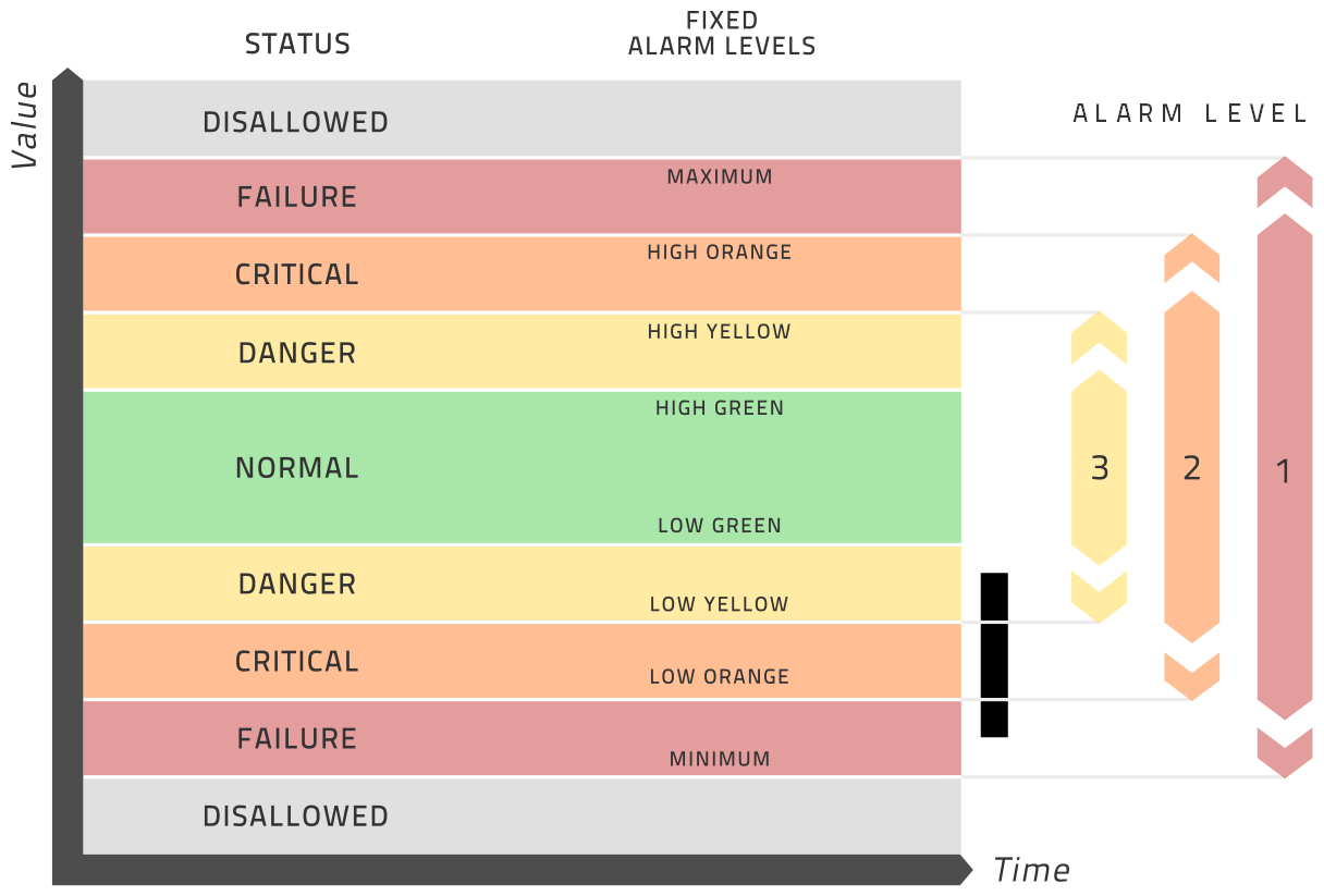
Optionally, you may specify up to three static alarm ranges for each measurement. This is provided so that IHM supports traditional condition monitoring in addition to its dynamic limit approach. This analysis and alarming is separate from the modeling analysis and thus totally optional. These ranges are best explained in the diagram below.
In summary, these are the initial choices to be made in relation to your dataset:
- Which tags are to be included?
- What data cadence is to be used?
- What time period will the dataset have?
- What are the time periods to be used for training?
- What exclusion conditions should be applied?
- For each tag …
- What is the allowed range of values?
- What is the tag uncertainty?
- Is this tag to be modeled and alarmed?
- Can this tag be directly controlled by the operator?
- Optionally, what are the static alarm ranges for yellow, orange and red alarms?
2.7. Software Architecture
The software has three major components. The central database that stores all data and model information is a PostgreSQL database. The data is analyzed by a command-line executable that reads data from the database and writes its results back to the database. The user interacts with this system via a browser-based graphical user interface written in Ruby-on-Rails.
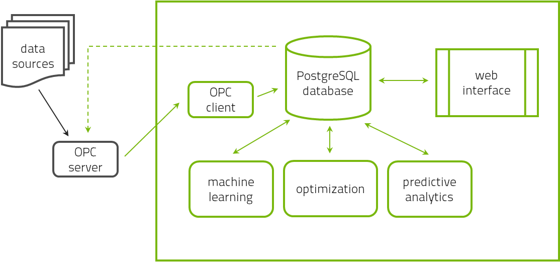
All three components are typically installed on a single computer-server on the premises of the users’ institution. All users can access the interface via any web-browser on any device connected to the intranet of the institution provided that the appropriate firewalls allow this access. As the software is installed on the premises, this is not a cloud service and the data remains on site. There is thus no security threat either by loss of proprietary data or hacking attacks.
The three components may be installed on different servers if the user desires to optimize the database server for disc space and the computational server for computation speed but this is not necessary.
Initially, the historical data is expected to be provided in the form of a file. The reason is that a data export followed by a data import has been found to be far more efficient rather than a direct data connection via e.g. OPC-HDA.
The regular reading of real-time data is done via OPC-DA. For this purpose, the name of the OPC server must be specified (an example is opcda:///Softing.OPCToolboxDemo_ServerDA.1/{2E565242-B238-11D3-842D-0008C779D775}) and any intermediate firewalls must be appropriately opened. Also, the full item name of each tag in the OPC server must be specified to be able to read the data.
3. How-To
This chapter describes various practical tasks independently of each other:
- Define the plant. In order to create a model, a plant must be setup and defined.
- Data preparation. The most essential task in advanced analytics is to prepare and describe the data to be analyzed.
- OPC connectivity. In order to analyze data in real-time, it must be connected to a data source by OPC.
- Bring Online. For real-time analysis, the application must be brought online.
3.1. Define your Plant
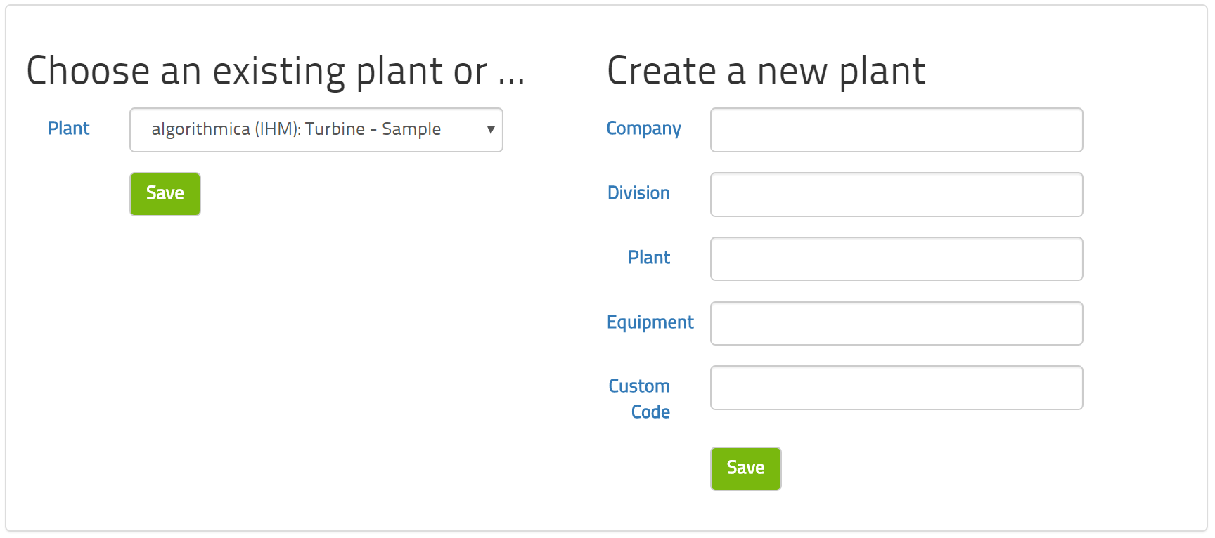
The plant is the entity that defines your data set. In order to construct a model, the first thing to do is to create a plant object for it.
In order to refer to the plant, you have four text fields available: company, division, plant and equipment. These are just labels so that you can organize several models in one user interface and manage user permissions to see individual models. You can also use the comment field to leave a longer note explaining what this model is about. During a testing or tuning phase, you may wish to construct more than one model in order to be able to compare them. The comment field is useful to keep track of which model was built how.
The custom code is a five-digit number provided to you by algorithmica technologies when you purchased the software licence for this plant. It's purpose is to identify any custom analysis steps that were written for you and included in the analysis software. If you are testing the software, you will not have this code and you may leave this field blank.
The maximum lag time is relevant only for use with the intelligent health monitor (IHM). The selection of independent variables used by IHM may be done automatically and may optionally include a time-delay. This option specifies the maximum time delay in number of time steps for this possibility. See the description of IHM modeling for more details.
The three fields OPC name, OPC DA version and subscription frequency are relevant for the OPC connection to a data source. This is relevant only for using the software in real-time. Please see the how-to section on bringing the system online for more information.
The three time periods that define the start and end of the reference time period and the start of the operational period are concepts used by APO to assess the success of the suggestions. The reference period is the time frame for the data used to build the model and the operational period begins when the suggestions made by APO are actually implemented.
3.2. Prepare Your Data
Machine learning works by analyzing historical data to find some pattern and to store that pattern in a mathematical model. For this to work, the methods require both the historical data itself and some extra information about the data. This section will describe how to prepare all this so that the learning can take place.
The situation that we want to model will generally have many properties that are measured by sensors and that we can include in the model. The first step is to choose which of the available sources of data will be included in the analysis. As a second step, each of these data sources needs to be characterized with some essential information such as its allowed range of values. The third and last step is to prepare a table of historical values for each of the data sources.
With all of this data in place, the analysis and learning can begin.
3.2.1. Select Tags
To start your modeling experience, please choose the tags to be included in the model. Your plant will have many sensors installed that measure a myriad of properties. Many of these will not be relevant for modeling. To guide your selection, please consider the following guidelines:
- Any tags that the operators regularly modify should go into the model.
- Any tags that represent important boundary conditions for the process should go into the model.
- Any tags that have relevance to security, quality, efficiency and monetary value should go into the model.
- Any tags that are used only during start up, shut down or emergency procedures are probably not relevant for modeling normal operations.
- Any tags that are used for condition monitoring or similar purposes are not relevant for optimization modeling.
As a rule of thumb, up to 90% of process instrumentation is irrelevant for modeling. In most cases, a process model only requires a few hundred tags even though many thousands may be available.
When in doubt, it is better to include the tag in the model. Too much data is always better than too little data. However, the model will be unwieldy and more time consuming to set up with an increasing number of tags and so it is in your best interest to keep the number of tags relatively low.
3.2.2. Prepare Meta-Data
When you have identified the tags you want to include, next you need to define some information about each tag. Most of these are straightforward.
There are two ways in which you can prepare this data:
- You can enter or edit the tag information directly through the interface by clicking on
plant -> edit tags. The form allows you to add tags or to edit the information for each tag. Please do not forget to save your work! This is the most convinient way to define this information. Please note that this table supports copy and paste but please be careful when using copy and paste for large amounts of information as there may be misalignments. - You can prepare a file that holds the information and is uploaded into the database in one go. This file will be a text file containing 16 TAB-delimited columns. If normal ASCII characters are sufficient, this file may be saved as ASCII but if non-ASCII (for instance the German umlauts ä, ö, ü or certain unit symbols such as ° or µ) characters are needed, then it should be saved in UTF8 encoding. This file may have a header row with the names of the columns in it.
Here follows a brief explanation of each column and whether it is required or not
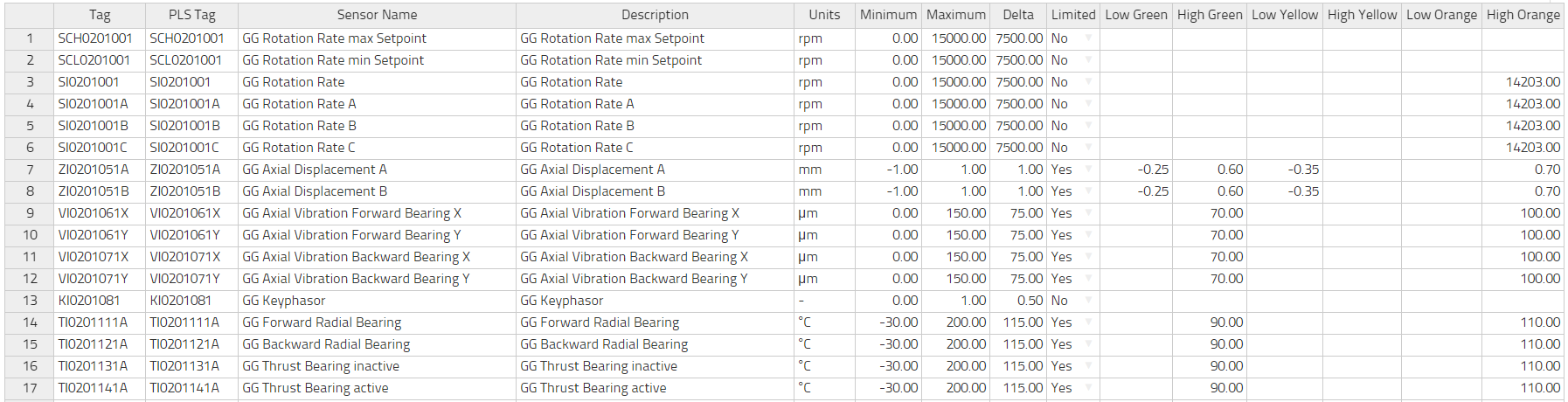
| Column Name | Requirement | Description |
|---|---|---|
| tag | required | The unique identifier for a time-series. This is often an alphanumeric string of characters used in the DCS or data historian to label a tag. |
| pls_tag | required | Often the same as the column "tag," this is the unique identifier used by the OPC server. algorithmica uses this column in order to query the current value of the tag from the OPC data source. It must therefore include any and all OPC item information. |
| sensor_name | recommended | A short description of what this tag is. |
| description | optional | A longer description of what this tag is. |
| units | required | The physical units of the tag, e.g. "°C" |
| minimum | required | The smallest value allowed. Any values lower than this will be ignored as not physically possible. For a detailed discussion on the concept of minimum and maximum see their section in the chapter on terminology. |
| maximum | required | The largest value allowed. Any values larger than this will be ignored as not physically possible. |
| controlability | required | Determines whether the tag can be directly controlled by the operator, not controlled at all, or indirectly controlled. |
| low green | optional | Within the range of allowed valued [minimum, maximum] we may define three sets of fixed alarm levels from the inside out: green, yellow and orange. Please see the image below for better understanding. |
| high green | optional | |
| low yellow | optional | |
| high yellow | optional | |
| low orange | optional | |
| high orange | optional | |
| delta | required | The measurement uncertainty of this tag in the same units as the value itself. If you are setting this up for the first time, please read the more detailed explanation of this concept in the chapter on terminology. |
| limit | required | This column is either "TRUE" or "FALSE" depending on whether this tag is to receive a dynamic limit from IHM or not. |
Columns that are not required, may be left blank. In particular, optimization by APO does not consider the colored limits. A sample file is provided with the installation files.
3.2.3. Prepare Process Data
The data file is an ASCII text file with its first column being a timestamp and then more columns of floating point numbers, one for each of the tags in the model. This file is semicolon-delimited. This file may have a header row with the names of the columns in it. It is essential that the order of the column in the data file is the same as the order of the rows in the tag file.
The timestamp may be in one of two formats:
- The standard European time format: dd.mm.yyyy hh:mm:ss.xxx
- The ISO 8601 format: yyyy-mm-dd hh:MM:ss.xxx
In both cases, the use of milliseconds '.xxx' is optional.
Here is a sample file that is semi-colon delimited.
| Time | CHA01CE011 | LAE11CP010 | LAE11CT010 | LBA10CF001 |
|---|---|---|---|---|
| 01.01.2015 00:00:00 | 1.1 | 2.1 | 3.1 | 4.1 |
| 01.01.2015 01:00:00 | 1.2 | 2.2 | 3.2 | 4.2 |
| 01.01.2015 02:00:00 | 1.3 | 2.3 | 3.3 | 4.3 |
| 01.01.2015 03:00:00 | 1.4 | 2.4 | 3.4 | 4.4 |
A sample file is provided with the installation files.
3.3. Setup OPC Connection
In order to update your model in real-time, the model must have access to the process data via an OPC interface. We assume that your control system, archive system or other data source provides an OPC server. algorithmica provides an OPC client in order to read this data.
The basic data of a plant (click on plant -> edit) includes three fields relevant to the OPC connection:
- OPC Name. This is the full name of the OPC server in your network. A sample name is opcda:///Softing.OPCToolboxDemo_ServerDA.1/{2E565242-B238-11D3-842D-0008C779D775}.
- OPC DA version. OPC includes several protocol types. algorithmica applications make use only of the DA type, which means data access. It is used to query the most recent value of a tag only. This protocol is available in version 2 or 3. Please specify which version your OPC server supports.
- Subscription frequency (sec). This is the number of seconds that we should wait before quering a new value. Please choose this number with great care. The application will query every tag at this frequency, store the values in the database and perform the model computations. Choosing a low number will not only strain the computational resources of your network but it will probably not achieve practical benefits as the human reaction time may not be sufficient to cope. Choosing a very large number may cause a significant time delay between the physical effect modeled and any possible reaction. In case of doubt, we recommend choosing a time period somewhere in the range of 300 to 900 seconds, i.e. 5 to 15 minutes. Ideally this value is the same as the data cadence chosen in the historical dataset.
If you have not done so already, please input these values into the interface and save them. We assume that you have already provided each tag with the field "PLS tag", which is the full OPC item name of that tag. The combination of the information of the OPC server and the OPC item of each tag allows the application to read the values.
Please note that the application computer must be able to access the OPC server over the network. This may require changes to be made to the firewalls in your network.
In order to check that the OPC server can be reached and that the items are read correctly, please go to plant -> OPC diagnostic. This form should display some basic information about the OPC server and also the current value of each tag. If there is a check mark next to the server status and each tag, then the connection is good and the item names have all been found. If there is an X next to server status, then either the server name is wrong or it cannot be reached on the network, please check with your network administrator. If there is a check mark next to server status but some tags have an X next to them, then their item names cannot be found on the OPC server. Please check these item names and correct them by going to plant -> edit tags
Having successfully provided all this information and checked it to be correct and working does not turn real-time computing on. You may turn real-time computing on and off independently of providing all the information required for its use.
3.4. Bring Application Online/Offline
In order to determine whether your application is currently running in real-time or not, please go to plants -> OPC on/off. The status displayed there will inform you whether the process is currently operating, when the last data point was read and what the update frequency of reading is set up to be.
Due to network delays and temporary communication breakdowns across computer networks, we have adopted the following definition of whether the OPC data connection is online: If the last data point read is at most two times the update frequency in the past, then the connection is considered online. If the last data point read is older than that, then it is considered offline.
Depending on the status, you will find a button to turn real-time processing on or off. After clicking on this button, please allow some time to pass before the connection is either established or severed. This may take several minutes depending on your network. By updating this page, you will eventually see the change in connection status.
This page also offers you the option to consult the OPC log file. This keeps a record of major activities on your OPC connection. There is usually no reason to consult this file unless there is a problem with the connection.
4. Advanced Process Optimizer (APO)
Operating a plant is a complex task for the operators who have to make many detailed decisions every few minutes on how to modify the set-points of the plant in order to respond to a number of external factors. The plant must always deliver what its customers demand and it must respond to changes in the weather and the quality of its raw materials among other things.
Plants are operated in shifts. A frequent observation during a shift change is that the new shift believes that it knows better than the previous shift. Therefore, a number of set-points are modified. The plant, due to its size, may require a substantial period of time to reach equilibrium after this happens. Some eight hours later, at the next shift change, the scene is repeated. As a result, the plant is rarely at the optimal point.
Not only is this true because of the divergent beliefs of the various shifts. It is also due to information overload as a plant may have ten thousand sensors that cannot possibly be looked at by human operators. So each operator must, by training and experience, decide which few sensors to use for their decision making. Those few sensors provide a lot of information but not all of it.
Automation and control systems are usually local and designed from the bottom up. They do well on encapsulated systems such as a turbine, furnace, boiler and such. An overarching methodology is very difficult for these systems and seldom considered. It is in the interplay of all the components of a plant that the potential for optimization lies untapped.
So let us consider the entire plant as a single complex system. It is a physical device and thus obeys the laws of nature. Therefore, the plant can be described by a set of differential equations. These are clearly very complex but they exist. This set of equations that fully describes the plant is called a model of the plant. As the model represents the physical plant in every important way, this model is often called a digital twin of the plant.
There are two basic ways to obtain a model. We might develop it piece-by-piece by putting together simpler models of pumps, compressors and such items and adding these into a larger model. This approach is called the first-principles approach. It takes a long time and consumes significant effort by expert engineers both to construct it initially and also to keep it up-to-date over the lifetime of the plant.
The second way to get a model is to start with the data contained in the process control system and to empirically develop the model from this data. This method can be done automatically by a computer without involving much human expertise. It is thus quick to develop initially and is capable of keeping itself up-to-date. This approach is called machine learning.
4.1. Process Optimization
The purpose of machine learning is to develop a mathematical representation of the plant given the measurement data contained in the process control system. This representation necessarily needs to take into account the all-important factor of time as the plant has complex cause-and-effect relationships that must be represented in any model. These take place over multiple time scales. That is to say that the time from cause to effect is sometimes seconds, sometimes hours and sometimes days. Modeling effects at multiple scales is a complicating feature of the data.
The model should have the form that we can compute the state of the plant at a future time based on the state of the plant in the past and present. This sort of model can then be run cyclically so that we can compute the future state at any time in the future.
The state of the plant is the full collection of all tags that are important to the running of the plant. Typically there are several thousand tags in and around a plant that are important. These tags fall into three categories. First, we have the boundary conditions. These are tags over which the operators have no control. Examples include the weather and the quality of the raw materials. Second, we have the set-points. These are tags that are directly set by the operators in the control system and represent the ability to run the plant. Third, we have the monitors. These are all the other measurements that can be affected by operators (as they are not boundary conditions) but not directly (as they are not set-points) and so adjust themselves by virtue of the interconnected system that is the plant as the boundary conditions or set-points change over time. A typical example is any vibration measurement. This data is used by machine learning to obtain a model of the plant's process.
Having gotten the model, we want to use it to optimize the plant's performance. Here we need to agree on a precise definition of performance. It could be any numerical concept. Sometimes it is a physical quantity such as pollution (e.g. NOX, SOX) released, or an engineering quantity like overall efficiency of the whole plant, or a business quantity like profitability. We can compute this performance measure from the state of the plant at any point in time.
So now we have a well-defined optimization task: Find the values for the set-points such that the performance measure is a maximum taking into account that the boundary conditions are what they are. In addition to the natural boundary conditions (e.g. we cannot change weather) there could be other boundary conditions arising from safety protocols or other process limitations.
This is a complex, highly non-linear, multi-dimensional and constrained optimization problem that we solve via a method called simulated annealing. The nature of the task requires a so called heuristic optimization method as it is too complex for an exact solution. Simulated annealing has some unique features. It converges to the global optimum and can provide a sensible answer even if the time is limited.
The procedure in real-life practice is that we measure the state of the plant every so often (e.g. once per minute) by pulling the points from the OPC server and then update the model, find the optimal point, and report the actions to be performed on the set-points. This can be reported open-loop to the operators who then implement the action manually or closed-loop directly to the control system. As soon as something changes, e.g. the weather, the necessary corrective action is computed and reported. In this way, the plant is operated at the optimal point at all times.
4.2. Correction and Validation Rules
When the machine learning algorithm learns the model, it retrieves the historical data from the database point-by-point. Each point is first corrected and then validated. Only valid points are seen by the learning method and invalid points are ignored.
Think of a valve and the tag that measures how open that valve is. A fully open valve records 100% openness and a fully closed valve records 0% openness. As a result, the minimum and maximum values for this tag are 0 and 100 respectively. However, we find in practice that due to a variety of reasons we do get numbers stored in the database that are a little below 0 or a little above 100. These are not really measurement errors or faulty points. We should not throw this data away but correct this data to what we know it to be. A measurement below 0 is actually 0 and a measurement above 100 is actually 100. We know this by the nature of the thing being measured and so we use a correction rule. Correction rules are rules that change the numerical value of a tag to a fixed value, if the value recorded is above or below some threshold. By default, there are no corrections applied to the data. If corrections are necessary, you must specify them manually.
The machine learning algorithm should only learn operational conditions that are reasonable in the sense that it would be ok if the model were to decide to bring the plant to that condition in the future. Any exceptional conditions that the plant was actually in at some point but should not really get into again, ought to be precluded from learning. Also any condition in which the plant is offline, not producing, in maintenance or any other non-normal condition ought to be marked invalid. A validity rule requires that a certain tag be within specified limit values. By default, every tag must have a value between its minimum and maximum for the point to be valid.
In addition to the default validation rules, we may manually add others. These additional rules do not have to always apply and so we can add a specification that this rule only applies when some tag is above or below a certain value. This applicability feature allows you to enter more complex rules depending on conditions. For example you could formulate the requirement that the process have a high temperature at full-load and a low temperature at half-load.
4.3. Goal Function
The purpose of process optimization is to tell you what set-points to modify in order for your plant to reach its best operating point. In order for this to be possible, you must define what you mean by best. Any numerical quantity will do, e.g. efficiency, yield, profit and so on.
APO will maximize the goal function and so it is important how you formulate your goal. If you want APO to minimize some quantity, e.g. cost, then all you need to do is to put a minus sign in front. Then maximization will turn into minimization.
All pieces of information needed to evaluate the goal function must be available in the database. Let's take the example of the revenue due to the sale of electricity. On the one hand, we need a tag that measures the amount of electricity produced. That is usually part of the process model anyway. We also need, however, the financial value of one unit of electricity sold. This is generally not part of the process model. In order to include it as part of the goal function, you must include this tag in the database as well. Please note that financial prices are generally tags of their own as prices do tend to change over time. That is to say, prices are generally not static numbers.
The goal function of APO is the sum of as many terms as you like with each term having three elements that are multiplied together:
- The factor is a number that is intended to convert any units that might need converting or to include any static multiplier needed for chemical reasons. It also offers the possibility to include a minus sign so that this term is subtracted instead of added to the goal function.
- The first tag is the main element of this term.
- The second tag is optional. Its main use is for a goal function that computes profit and so we need to multiply volume by price in every term.
The input form allows you to specify a time period over which to evaluate the goal function's terms and add them up to their total. This is just for checking and will not influence the model in any way. Please use this feature in order to check the plausibility of the values. In practice, we often find that tags are recorded in different units than expected (for example tons instead of kg) and this causes rather large deviations in numerical values. In addition, sometimes a corrective factor is needed for the molar mass of a substance.
Each tag used in the goal function should ideally be semi-controllable. If a tag is controllable, then the optimizer can simply set it to its maximum value. If a tag is uncontrollable, there is nothing that can be done about that aspect of the goal anyway. This is a guideline and not a strict requirement however. If it is necessary, for the correct computation of profits, for example, to include some uncontrollable tags, then that is necessary.
The goal function is the centerpiece of APO that guides every decision. This must be specified with great care. If this function corresponds to your true business goals, then APO will get you there.
4.4. Train the Model
Training the model is an automatic process. You can trigger the training of the model either via the APO Wizard or via the APO Menu by selecting the Model option.
The form will ask for you to select the method you would like to be applied. Both choices will delete the current model and create a new one from the historical data. Method Model only will just do that and nothing more. It will therefore keep all the suggestions already made and all the manually entered reactions from the operators. This option is the right one for you if you have had APO in active use for some time and you merely want to update the model but retain the suggestions made in the past. Method full recomputation will also delete all suggestions made along with any manual reactions to suggestions. It will then recreate them all after the model is finished. This is the right option to choose if you are deploying APO, using it for the first time or in the process of fine-tuning the model.
The time limit can be used to speed up the recomputation of all historical suggestions by only computing them from the begining of known history to the specified point in time. Generally, we do not recommend using this option and recommend modeling the entire dataset.
Please note that training can take a substantial period of time. The amount of time is directly and linearly proportional to the number of data points in the database. The process is dominated by the read/write speed of database operations and thus the speed of the hard drive. Please be patient.
At the end of training, the model is saved in the database. If you have selected full recomputation, you will be able to look at the newly computed suggestions and assess model quality. We strongly recommend that you do so.
4.5. Assess Model Quality
There are three steps to assessing the quality of a trained APO model:
- Checking plausibility
- Reading the model report
- Fine-tuning the model
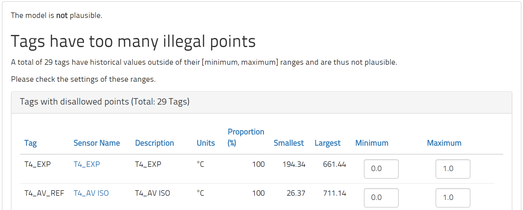
The model plausibility looks at the historical data in relation to the specifications made for each tag and tries to assess if these specifications make sense. The first thing checked is the measurement range of each tag. From the historical data, it is computed how many points lie inside and outside of the interval from minimum to maximum. This interval is intended to mark any and all normal and reasonable values. Therefore, only a very small minority of historical observations should lie outside this interval. However, we frequently find that some tags have a great many points outside this interval.
The minimum and maximum values are important because any point outside this allowed range is excluded from modeling. Generally, these values need adjustment before enough valid points are available to train a sensible process model. In the plausibility form, you will see not only the percentage of historical points that lie outside this interval but also the smallest and largest values ever measured for this tag. This information should help to guide you in making the appropriate corrections.
The second check concerns the measurement uncertainties of the uncontrollable tags. The modeler clusters the available historical data on the basis of the measurement values and uncertainties of the uncontrollable tags. For each such cluster, a separate optimization model is built. This is done in order to avoid suggesting a operational condition that cannot be reached because one or more of the uncontrollable tags are different. As they are uncontrollable, they mark boundary conditions to the process. The more tags are marked as uncontrollable and the smaller their uncertainties are, the more restrictions are put on the model. A more restrictive model will be able to optimize less.
In this check, please examine the selection of uncontrollabel tags. Perhaps some of them can be removed from the model if they do not really represent a boundary condition. Please also have a look at the uncertainty of these tags. The plausibility form will tell you how many clusters are formed on the basis of this tag. If in doubt, please start with larger uncertainty values to obtain a reasonable model. This can always be lowered at a later time to make the model more restrictive.
The third plausiblity check concerns the validity of historical data. Only valid points are used for training. A point is valid if all controllable tags are within their minimum to maximum ranges and if all validity rules are satisfied. You may also have defined a number of custom conditions that must be met. A common such custom condition is to require the plant to achieve a steady-state for validity. This effectively excludes all transient states from learning. If we have very few valid points in the history, then there may be too little data to learn from. As a plant's operations should generally be normal, having few valid points indicates that some settings need correcting.
After these three checks have been passed, the machine learning should be able to train a reasonable model for your process. Please train the model and have a look at the model report next.
4.6. Understand the Model Report
After you have trained the model, you can have APO generate a model report. This is either the last step in the APO wizard or you can get to it via the APO menu choosing the report option. The report generator asks for a time period and a granularity of the report. By default, the time period is set to the entire time period for which data is in the database. The report will be compiled for that time period and statistics will be collected with the frequency specified by the granularity.
The report itself contains an explanation of its data tables and diagrams. The report is mainly concerned with analyzing the optimization potential provided by APO. Every suggestion provides an opportunity to improve the plant's performance. If that suggestion is implemented, then that opportunity is realized as a actual gain. These opportunities and realized gains are summarized in the report. Please check that the magnitude of improvement is realistic. If the improvement is very large, the model may not know about all the restrictions or boundary conditions that the process has. If the improvement is very small, perhaps the restrictions on the model are tighter than they are in reality. A more detailed analysis of the suggestions themselves follows in the process of fine-tuning but an assessment of the rough numerical size of improvement should be done now using the report.
The report will also contain a list of the most common suggestions made. A single suggestion may contain several lines of changes to be made. Each of these changes is averaged out here and sorted according to how often they appear. You will see how often tags are changed and by what average amount they are changed. This average is supplied with a standard deviation so that you can see how much variation about this average takes place. Tags that appear in nearly every suggestion probably have an uncertainty that is too small and thus make nearly every value sub-optimal. Tags that appear in hardly any suggestion may not have a great influence on the process and perhaps should be ignored. On the other hand, they may have an uncertainty that is too great as to hide the true influence they may have. If the changes are often very large, perhaps there are limiting factors that must be imposed on the model.
4.7. Fine-Tune Your Model
After you have built a model and it is essentially sound on the basis of the tag settings, plausibility check and the model report, it is time to perform model fine-tuning. This is a process that may take some time and involves looking at many individual suggestions but will eventually make the model ready to be used in practical work and will also provide the confidence to use the model.
In the APO menu, please choose the option of fine tuning. To first begin fine tuning for a plant, please click on the button Initialize. This will select 100 randomly chosen historical suggestions for your review. These will then be listed in the fine tuning overview. You can restrict the list by using the form and clicking the button Filter. Filtering may be done by either the time of the suggestion or whether this suggestion is marked ok or not ok. Initially, of course, all suggestions are marked not ok.
Please now look through each suggestion carefully. Note that this suggestion was made a particular time in the past in response to a very particular state of the plant and its environment. In your assessment of the suggestion, please recall this situation. The questions to ask with each suggestion are
- Could all the listed changes have been implemented at all?
- Are there any reasons for not implementing any of the changes?
- What settings in the model need to be changed in order to prevent unrealistic changes from being suggested?
A suggestion is fairly self-explanatory. Please note that each suggestion only suggests to move the plant into a condition that it has already experienced at least once in the known history. This previous experience occured at a time that is labeled "Prior at" in the table. If you click on this timestamp, a comparison page will appear giving you the details of the current and this historical point so that you may compare them. This is useful for understanding what the model sees as a comparable condition and thus perhaps making modifications to the model or simply understanding where the suggestion comes from.
When you have checked through all the suggestions and collected a number of alterations to be made to the model, please actually make these alterations and retrain the model using the option of full recomputation. This will recompute all suggestions. Then go back to the fine tuning overview and now click on the button Update. This will now get the new suggestion for all the specially selected fine tuning suggestions you have already looked at.
Look though all the suggestions a second time. The ones marked ok, should still be ok. The ones marked not ok, could now have improved. If they are ok now, please mark them ok. This process should repeat until all suggestions in the fine-tuning overview are marked ok. At this point the model has been adjusted for a significant and representative sample of historical suggestions to be practical and good.
You can review your work done by clicking on Overview that will supply you with a quick count of the number of suggestions marked ok during every iteration of this process. You can also click on Report to get a full (and lengthy) report on the evolution of every suggestion and all your comments.
At the end of fine tuning, the model is ready to be used in real plant operations. We recommend using the model for a few days in probationary capacity just in case some feature only becomes apparent in current operations.
5. Intelligent Health Monitor (IHM)
The Intelligent Health Monitor (IHM) makes condition monitoring smart by bringing it into the age of machine learning. Normal condition monitoring suffers from giving false alarms, not alarming all bad conditions, and requiring significant human expertise to set up and maintain. IHM solves all three of these problems by providing effective, efficient and accurate methods to detect equipment health. This is done by changing the definition of health from human specified limit values for each tag separately to a holistic form based on the past performance of the equipment.
Unhealthy states are detected because the combination of various measurements is taken into account by the holistic modeling approach. For example, temperature, pressure and rotation rate give valuable information about whether the vibration is acceptable or not. Due to that approach false alarms are also avoided. As the method is based on historical data, maintenance engineers no longer have to specify, maintain and document alarm limits.
As a result of the increased reliability of health detection, the availability of the equipment and thus the plant increases. With the increased availability, the effective production capacity of the plant improves. Due to being able to proactively maintain the equipment, maintenance can increasingly be planned and thus becomes less expensive. As the equipment no longer fails but can be proactively repaired, collateral damage is avoided and significantly lowers maintenance expenditure.
5.1. Condition Monitoring
In operating technical equipment in an industrial plant, we are concerned whether this equipment is in good working order at any one time. Activities concerned with determining this health status are grouped under the term condition monitoring. This is generally approached by installing sensors on the equipment measuring quantities like vibration, temperature, pressure, flow rate and so on. These measurements are transmitted to the control system and usually stored in a data historian.
In between the control system and the historian, the data is analyzed to determine the health status of the equipment. For this purpose, one usually defines an upper and lower alarm limit for each tag of importance. If the measurement ever goes above the upper limit or below the lower limit, an alarm is released.
When an alarm is released, a maintenance engineer looks at the data and determines what, if anything, must be done. If the engineer determines that nothing must be done, the alarm is a false alarm. If the equipment is not in good working order but this status is not alarmed, this is called a missing alarm. Both are problematic. The false alarm is unwanted because it wastes time and resources. The missing alarm is dangerous because it will most likely result in an unplanned outage that may cause collateral damage and production loss.
The reason for both false and missing alarms is usually due to the simplistic nature of the analysis. The static nature of the upper and lower limit is not able to capture the complexity of diverse operating conditions of industrial equipment. In addition, the fact that each measurement is analyzed individually is a major drawback. All measurements on a single piece of equipment are obviously connected. By ignoring this natural connection, the analysis is throwing away a major source of information.
One may try to overcome the first defect by what is known as event framing. This is where one defines certain operating conditions of the equipment as belonging to one group and then supplies an upper and lower limit only for that group. For example, one may divide the data from a turbine into full load, half load and idle conditions by defining a condition on the rotation rate. While this is a certain improvement, it also increases the amount of manual work that must be done to setup and maintain the analysis. With plants having tens of thousands of measurements, this quickly becomes overwhelming and error prone.
We conclude that normal condition monitoring defines the health of a piece of equipment measurement-by-measurement through specifying limiting values based on human engineering expertise. This definition of health is limited in its effectiveness and requires significant human effort both initially as well as continually.
5.2. Concept of Dynamic Limits
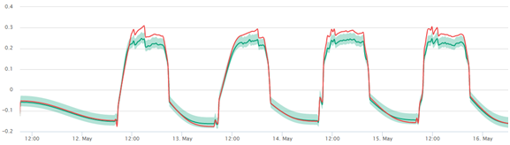
IHM constructs a machine learning model of one measurement time-series as a function of several other such time-series coming from one industrial plant or piece of equipment. If the underlying physics and chemistry of the industrial process remains the same over the long-term, then the modeling process will be able to deliver an accurate, precise and reliable model for the measurement concerned.
This model is constructed over a time period where the equipment is known to have been healthy. Therefore the model becomes the definition of health for the tag being modeled instead of the static limits in normal condition monitoring.
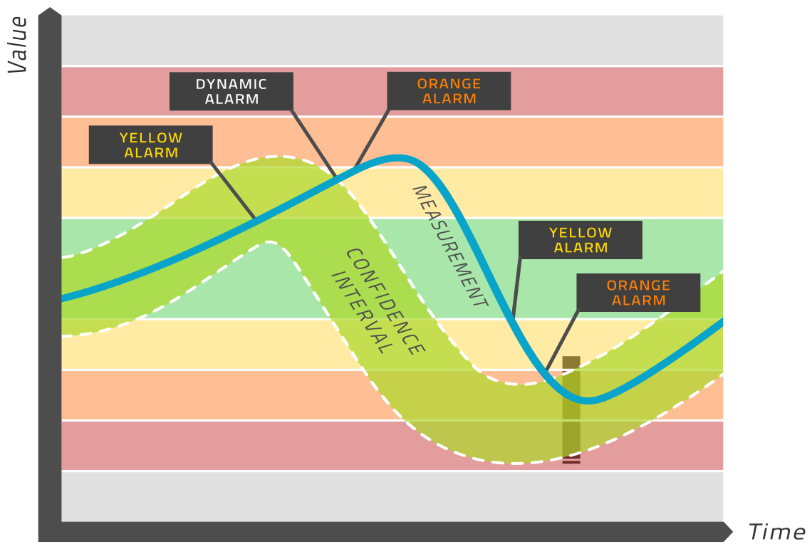
The model is evaluated in real-time and yields an expected value for each relevant tag. A confidence interval is computed around this expected value, which amounts to a range of values (light green band in the above picture) that are considered healthy. If the measured value lies within this band, then the equipment is healthy. If the measured value is outside this band, then an alarm is released. This is in sharp contrast to normal condition monitoring, where alarms are released based on limiting values that do not change over time, such as the normal yellow, orange, red regions that one can define in many condition monitoring tools. This is why we refer to this approach as dynamic limits. Please see the image above for a visual depiction of this process.
If you are interested in the model itself and how it is obtained, please see below in the section on mathematical background.
5.3. Concepts of IHM
Machine learning methods take empirical data that has been measured on this particular machine in the past when it was known to be healthy. From these data, the machine learning methods automatically and without human effort construct a mathematical representation of the relationships of all the parameters around the machine.
It can be proven mathematically that a neural network is capable of representing a complex data set with great accuracy as long as the network is large enough and the data consistently obeys the same laws. As the machine obeys the laws of nature, this assumption is easily true. We therefore use a neural network as the template for modeling each measurement on the machine in terms of the others. The machine learning algorithm finds the values for the model parameters such that the neural networks represent the data very accurately.
The selection of which measurements are important to take into consideration when modeling a particular measurement can also be done automatically. We use a combination of correlation modeling and principal component analysis to do this.
The result is that each tag on the machine gets a formula that can compute the expected value for this tag. As the formula was trained on data known to be healthy, this formula is the definition of health for this machine. Unhealthy conditions are then considered deviations from health.
It is important to model health and look for deviations from it because health is the normal condition and much data is available for normal healthy behavior. Rather little data is available for known unhealthy behavior and this small amount is very diverse because of a host of different failure modes. Failure modes differ for each make and model of a machine making a full characterization of possible faults very complex. Modeling poor health is not a problem of data analysis but rather data availability. As such, this problem is fundamental and cannot be tackled in a practical and comprehensive way.
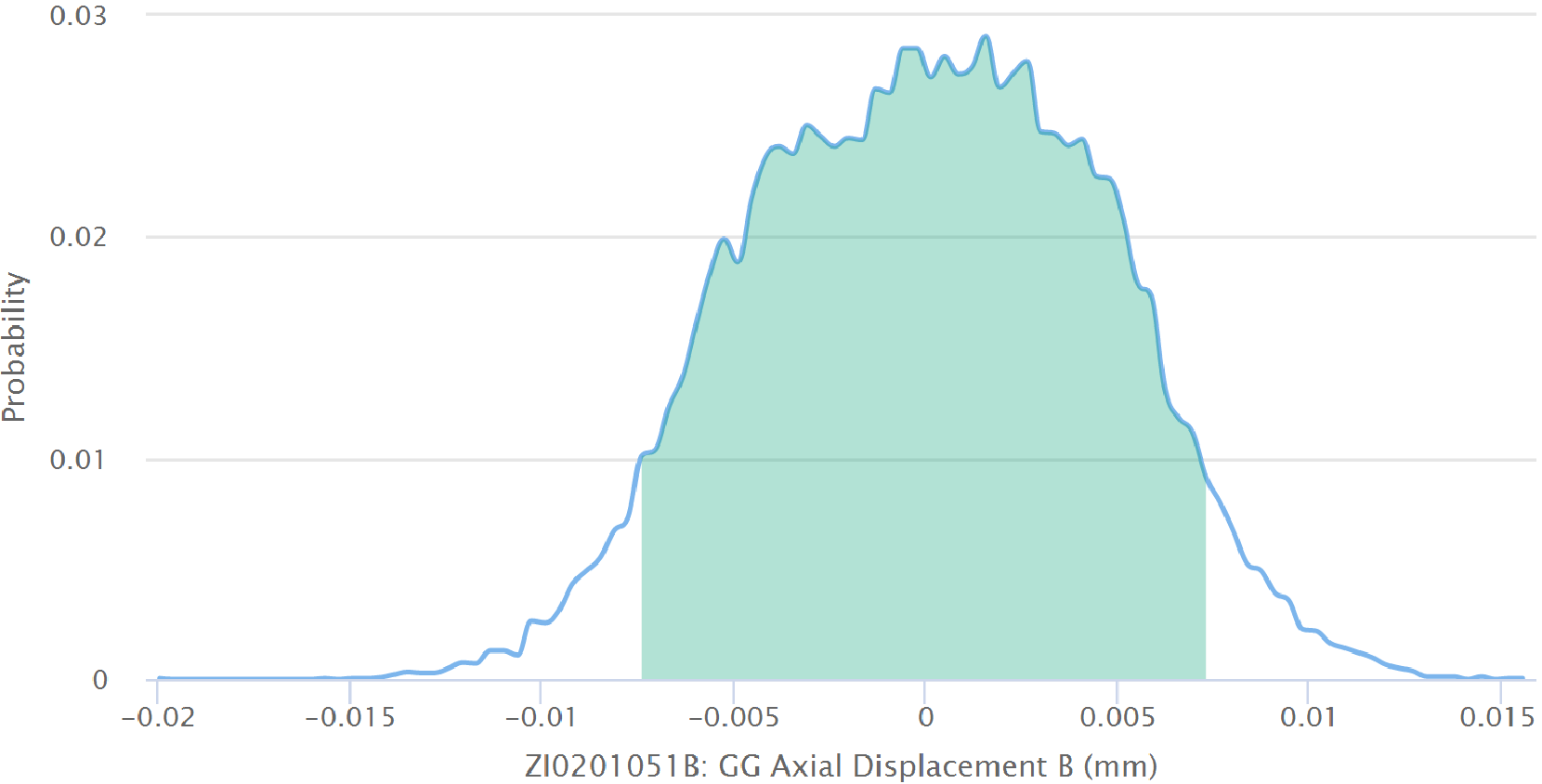
At any one time, we can compare the expected healthy value to the sensor value. As the expected value is computed from a model, we know the probability distribution of deviations, i.e. how likely is it that the measurement will be away from the expectation by a certain amount. So we may compute the probability of health from this distribution or conversely use this confidence interval in order to judge if the sensor value is too far away from health. If that is found to be the case, then an alarm is sent.
The alarm can be enriched by the information of how unhealthy the state is by providing the probability of poor health. Since the expected value has been computed from a (usually small) number of other machine parameters, it is generally possible to lay blame on some other measurement. This gives assistance to the human engineer receiving the alarm in the effort to diagnose the problem and design some action.
With normal condition monitoring, in practice, it is often found that when a machine transits from one stable state to another, lots of (false) alarms are released because a simple analysis approach cannot keep up with the quickly changing conditions. As a neural network can easily represent highly non-linear relationships, even a startup or load change of a machine will be modeled accurately without alarm if everything is as it should be.
5.4. Initial Putting into Service
After installing IHM on your system, you will find a menu on the interface page. One of the entries is called Wizards and among them is the IHM Setup wizard. If you click on this, you will be guided through a workflow to generate a new dataset with model and dynamic limits.
First, you generate a new plant. While this is called a plant, you may want to create a new plant for each major piece of equipment. The decision which data points belong into a single analysis framework, here referred to as a plant, is up to you and depends on how connected these parts are. The IHM software can handle multiple plants.
Second, you define the measurements and their metadata. This is explained in the wizard in detail. You may enter this information directly in the form on the page or you may prepare the information externally and put it into a file.
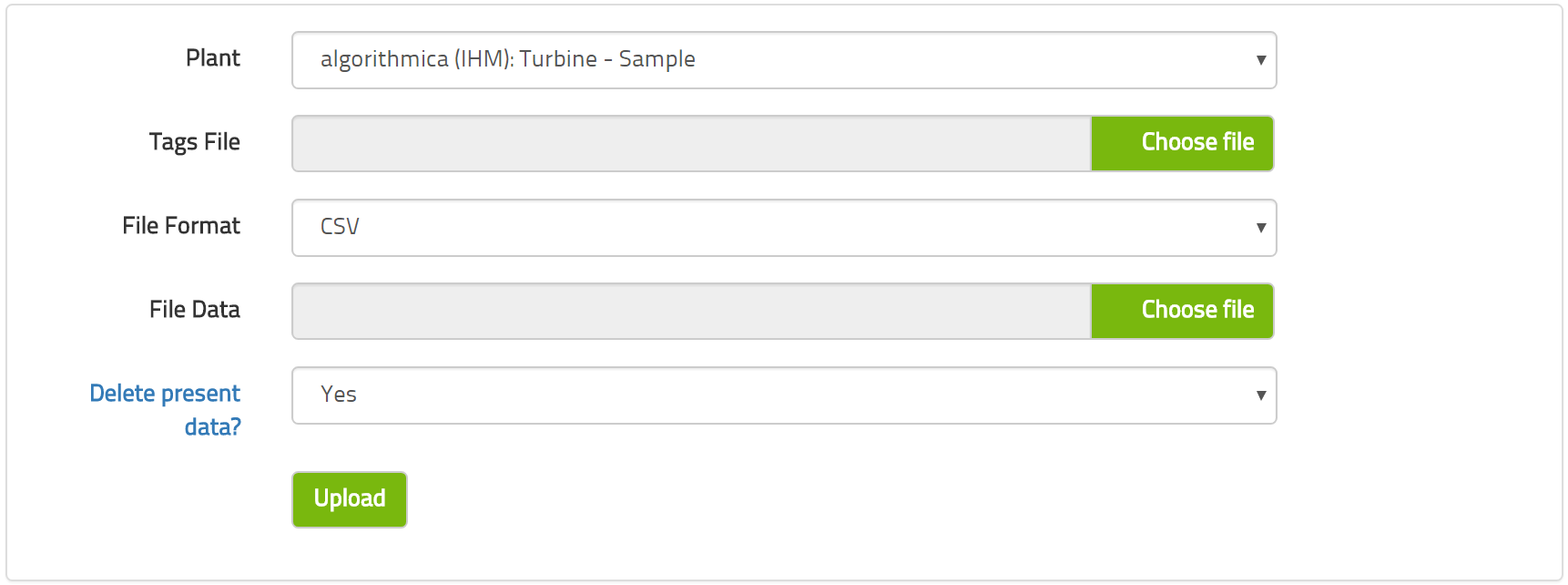
Third, you will upload the historical data that you have exported from your data historian. Here you will also upload the metadata if you have not manually typed it into the online form before.
Fourth, there will be a plausibility check for the metadata. If there are any implausibilities, the interface will explain what they are and how to fix them. This essentially detects any typos in the ranges of values and so on to make sure that everything makes numerical sense.
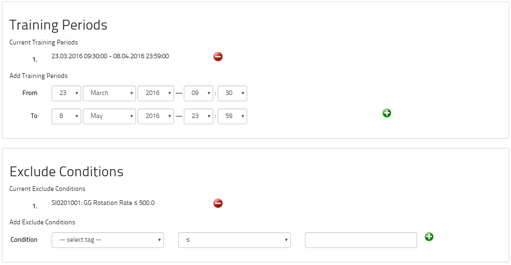
Fifth, you can enter the time periods that the equipment was known to be healthy and any exclude conditions. These two wizard entries will apply to all models for this dataset. You can, if you wish, customize these two pieces of information for each model individually. It is far more efficient to do it here globally. It makes sense that the times of health apply to the whole equipment and that exclude conditions also apply for the whole equipment. Thus, we recommend that you only customize these concepts for each model in exceptional circumstances.
On this last page, there is a button to model everything. If you click on this button, the computer will automatically select the independent variables, train and apply the model to the historical data for every single model requested in the metadata. Depending on the number of models requested and the amount of training data, this may take a substantial period of time. We recommend pressing this button at the end of a working day or even on a Friday afternoon so that the computer may work for many hours without disturbing you during any other items of work.
5.5. Creating or Customizing the Models
We recommend following the IHM setup wizard in order to initially work with a new dataset. It is recommended to have a look at each model to check if it is good or not. Instructions for goodness of fit can be found in the section on mathematical background.
When you enter the edit page for a particular model, you will find that you can modify the training times and add exclusion criteria. We recommend that you do not do this but rather edit this information globally for the entire dataset using the IHM wizard. Changing this information for an individual model should be done only in exceptional circumstances.
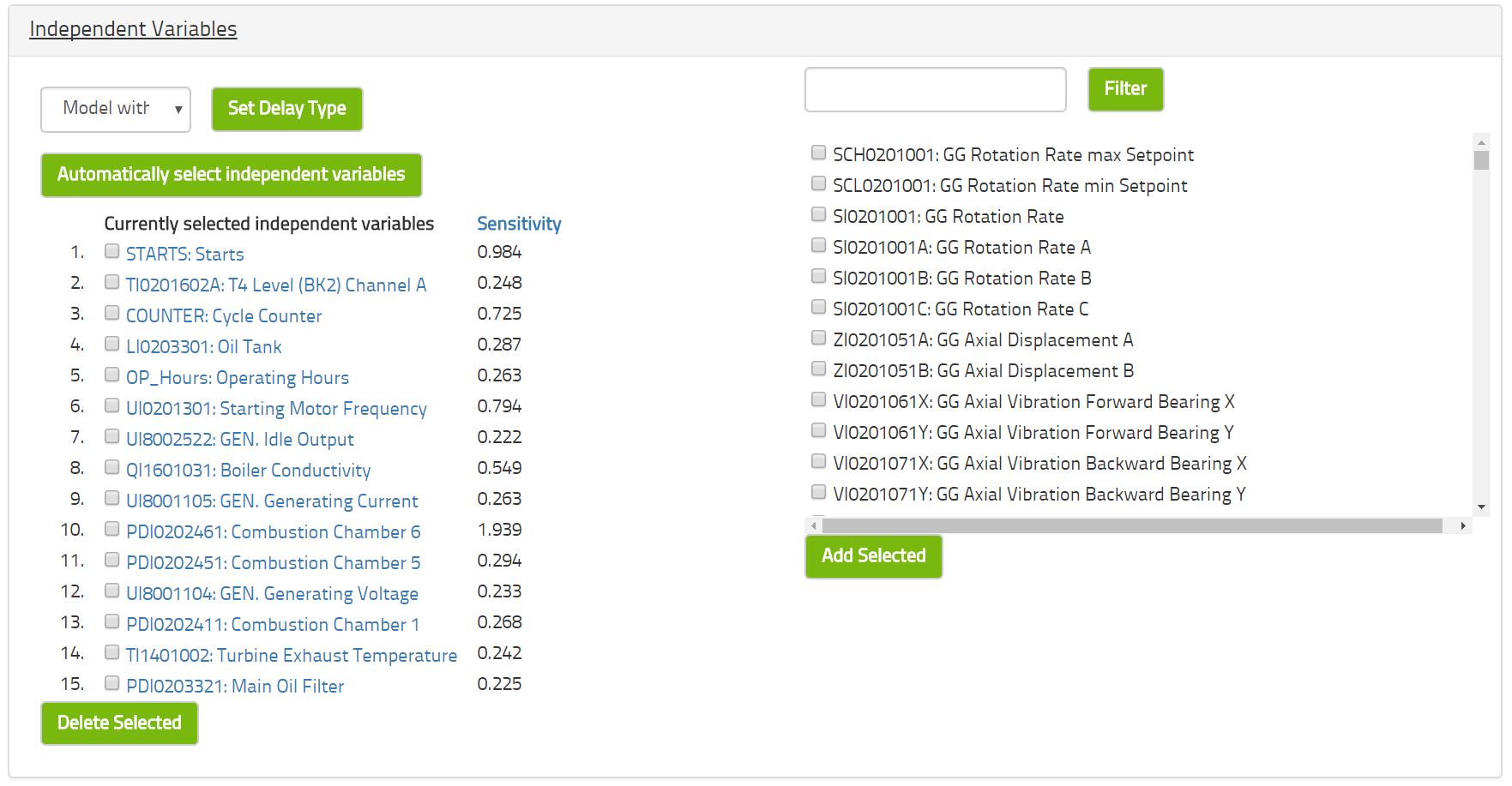
You may alter the selection of variables by either deleting or adding variables to the list of independent variables. You may also change more advanced settings such as the confidence level desired or the number of neurons in the neural network. The confidence level defaults to 0.9 and the number of neurons defaults to twice the number of independent variables. Please see the section on mathematical background for more details on these concepts.
Having made these changes, you will find three buttons at the bottom of the page. They will model, apply or do both (model and apply). Model means that the model will be retrained using the current settings and stored in the database. Apply means that the model will be executed on the historical data thus recomputing historical results and alarms. Generally, you will want to both model and apply.
If you only model, the historical results and alarms will be kept. This is interesting only if you have already been working with the system in an online capacity and need to retain the historical alarms for reporting purposes. If you only apply, then the model will be executed as it is. If the model has not changed, this will just reproduce the same results but will first delete the alarm history alongside and any manual alarm editing that you may have done.
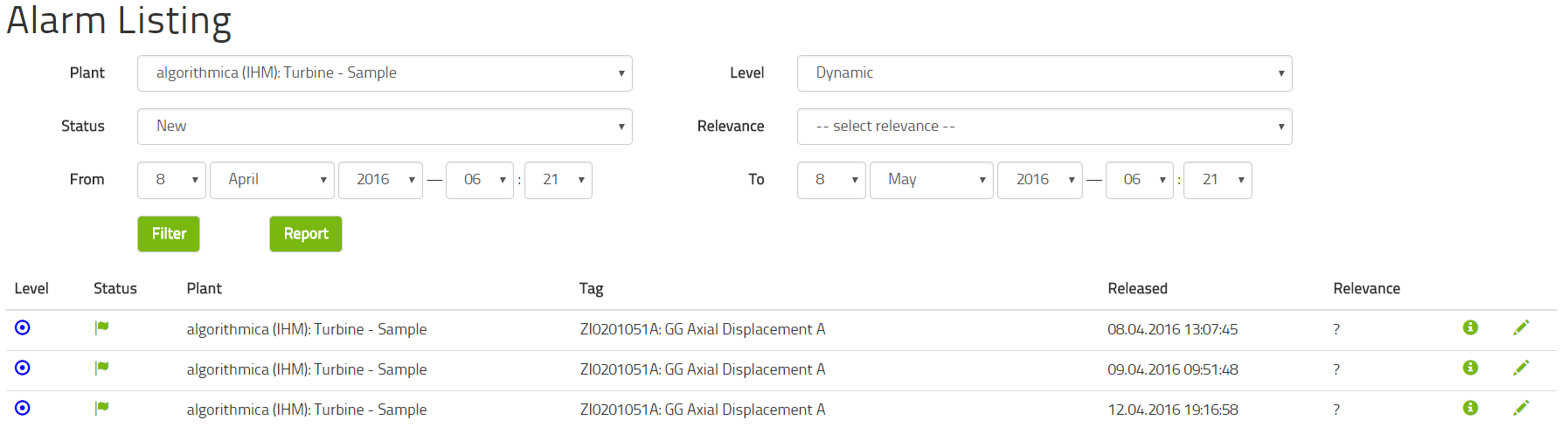
5.6. Getting and Administrating the Alarms
Having modeled and applied the model, the application will have computed any historical alarms. These can be looked at using the menu for IHM and Alarms. To select the right alarm you are interested in, you may use several filters and then obtain a list of alarms.
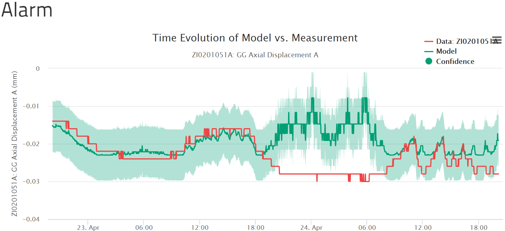
If you click on any one alarm, you will see a brief report about the alarm including a relevant chart of the alarm for 24 hours before and after the alarm.
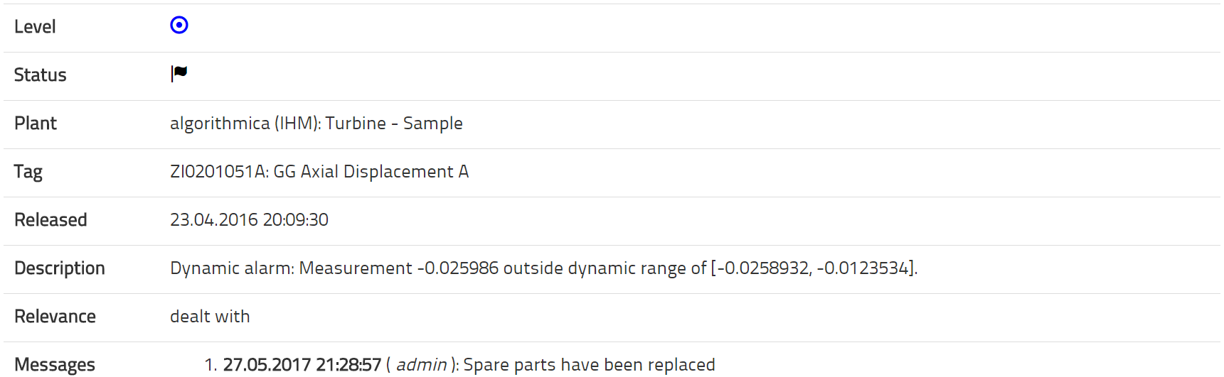
If you click on edit, you may change the category of the alarm and add messages. This information can be retrieved by looking at this alarm or producing an alarm report that may be useful for periodic documentation.
6. Intelligent Soft Sensor (ISS)
Sometimes it is difficult or expensive to measure a quantity of interest by a sensor installed in the process. In that case, we might opt to measure it manually by a hand-held sensor, a portable devise or by taking a sample and having it investigated in the laboratory. This manual process becomes tedious and expensive in its own right after some time. Additionally, the value only becomes available when we perform this process and even then only with a delay.
A soft sensor is a piece of software intended to replace the manual measurement process by computation. The value is available in real-time without making any manual effort. This can be used to compute process efficiency, gas chromatography, pollutants or any other quantity hard to measure.
The soft sensor is a essentially a formula that computes the quantity of interest from other quantities that can be measured in the normal way. The formula itself is determined using machine learning from the data collected by hand. First, the computer determines which process values are necessary to compute the interesting one. Second, the data is collected and a model is trained. Then the model quality can be checked and the model can be improved, if necessary. Once the model is good, it can be deployed computationally in order to look just like any other sensor.
6.1. Creating a new Soft Sensor
In the ISS menu, you can access the list of all soft sensor present in your plant. The button at the bottom will lead you to a page for creating a new soft sensor. The tag is the tag that contains the manually collected data for the quantity of interest that you want to model. The new tag is the alphanumeric nomenclature for the new tag that will be the result of the formula about to be constructed. We recommend that this nomenclature be very similar to the nomenclature of the original tag but it must be a unique identifier for this plant. When you click on Create, not only will a new soft sensor object be generated but a new column will be added to the table of historical data for your plant. This new column is for the computed data from the new soft sensor.
You will be taken to the edit page for the soft sensor. First, you will need to define one or more training time periods that select the historical data on which the soft sensor is to be trained. From these time periods, any points will be excluded that match any of the exclude conditions that you can also define here. Both of these elements together will result in a list of data points that will be used for training.
Next, comes the selection of independent variables. These are the variables that go into the formula that will eventually compute the value of the soft sensor. If you know what tags influence the quantity of interest, you can manually select them and add them to the model. However, we do not recommend that you do so. There is a button to perform this selection automatically by virtue of data analysis. It is preferable to do any manual editing after the automatic selection process.
Having selected the variables that are going to go into the model, we may edit some more parameters of the model. The soft sensor can be given a name and you can write a comment text on it, if you would like. More importantly, you can edit the number of hidden neurons. The formula for the soft sensor will be a neural network. Hidden neurons are essentially the free parameters in this formula. The more hidden neurons one has, the more free parameters one has. Having more parameters usually allows the model to fit the training data better but only up to a point. There is a law of deminishing returns at work here and also there comes a point at which the number of parameters is so large that the training data can be memorized rather than learned. At this point, the model can reproduce past data with perfection but it cannot generalize to a new situation at all well. We recommend choosing a number of hidden neurons equal to approximately twice the number of independent variables.
After setting all this up, you are ready to construct the model. The button Model trains the model, the button Apply uses the model, computes the value of the soft sensor for the entire available history in the database and saves these values there, and the button Model and Apply does both of these things in one operation. We recommed to model and apply together. You can then go to the show page in order to examine how good the soft sensor is.
6.2. Assessing Model Quality
Navigate to the show page for your soft sensor. You will be taken there automatically after you have pushed the model and apply button on the edit page or you can select the show link on the list of soft sensors accessible through the ISS menu.
On the top of the page, you can select a time period for the time series display. This will select data for the original tag and the soft sensor tag over this time period and display it in two ways. The top diagram will be a simple time-series plot and the second diagram will plot the measured value against the computed value. Ideally the two tags will have equal values. Realistically, they will differ at least by some inherent random variation that is a result of the measurement process. On the plot of both tags versus each other, you will find a straight black line. This is the ideal line you would get if both values were always perfectly equal. Based on this line, you can judge the degree to which they agree.
The third plot is the probability distribution of the differences between the modeled and measured values. Ideally, this is a bell-shaped curve with its center at zero deviation. The curve should be symmetrical about its center and be sharply peaked. Look at where the bell shaped curve drops off on either side. There is a point at which the sharp descent from the center turns into a gentle approach to the axis; this is the "elbow" of the distribution. If this elbow on either side occurs at a difference value comparable to the measurement uncertainty of the original tag, then all is well. Should this plot have more than one significant and pronounced peak in it, then the model has a systematic problem that is almost certainly the result of a sub-optimal selection of independent variables, i.e. the model is lacking an important source of information.
Further down the page, you can see some statistical quantities to make this assessment more precise. If you are not convinced of the model's quality, please edit either the training time periods, the exclusion rules, or, most importantly, the selection of independent variables. As a last resort, you could increase the number of free parameter by increasing the number of hidden neurons. Please note that it is possible for an independent variable to be a source of disinformation that could harm model accuracy. Consider making a soft sensor for the NOX emission of a power plant and using your heart rate as an independent variable. At best, this will have no effect on the model but it is more likely that the model will suffer because your heart rate adds structure to the data without any causation.
In the exceptional case that you have carefully checked the selection of independent variables as well as all other settings and still get a poor model, then you may conclude that there is a essential piece of information in your process that you are not currently measuring or have excluded from the model.
.
7. Background and Concepts
A mathematical model is a mathematical description of a system that usually takes the traditional equation format, e.g. y = mx + b.
Modeling is a process that has the mathematical model as its objective and end. Mostly it starts with data that has been obtained by taking measurements in the world. Industrially, we have instrumentation equipment in our plants that produce a steady stream of data, which may be used to create a model of the plant. Note that modeling itself converts data into a model -- a model that fits the situation as described by the data. That's it.
Practically, just having a model is nice but does not solve the problem. In order to solve a particular practical problem, we need to use the model for something. Thus, modeling is not the end of industrial problem solving but modeling must be followed by other steps; at least some form of corporate decision making and analysis. Modeling is also not the start of solving a problem. The beginning is formed by formulating the problem itself, defining what data is needed, collecting the data and preparing the data for modeling. Frequently it is these steps prior to modeling that require most of the human time and effort to solve the problem.
Mathematically speaking, modeling is the most complicated step along the road. It is here that we must be careful with the methodology and the data as much happens that has the character of a black box.
Generally speaking modeling involves two steps: (1) Manual choice of a functional form and learning algorithm and (2) automatic execution of the learning algorithm to determine the parameters of the chosen functional form. It is important to distinguish between these two because the first step must be done by an experienced modeler after some insight into the problem is gained and step two is a question of computing resources only (supposing, of course, that the necessary software is ready). In practice, however this two-step process is most frequently a loop. The results of the computation make it clear that the manual choices must be re-evaluated and so on. Through a few loops a learning process takes place in the mind of the human modeler as to what approach would work best. Modeling is thus a discovery process with an uncertain time plan; it is not a mechanical application of rules or methods.
7.1. Concepts
7.1.1. Concept of a Model
A model of a measurement is a formula that computes that measurement from other data such as other measurements. A simple example is the well-known ideal gas law from thermodynamics PV = nRT. For an ideal gas, this formula relates the pressure P and volume V to the temperature T and the amount of the gas n. The relationship depends on a parameter R that must be determined in some other way. This is called the ideal gas constant and is known to be a universal constant that can be determined by experiments. The fact that this law applies to real physical systems can be motivated by theory and determined by experiments in practice.
As a practical application, we could easily measure the volume, pressure and temperature of our gas and determine how much gas is in the vessel using this formula without having to measure that via some complex flow measurement. Such a model is thus useful in practice if we have the data for the other unknowns.
This is where we have to review a bit of vocabulary. We call something a variable if we have to determine it by measurement or computation because it changes over time, e.g. pressure or temperature. Other things are called parameters because they stay constant and require determination only once, e.g. the ideal gas constant. A variable is dependent if this is the variable we want to compute from other variables that are then called independent. It is the independent variables that must be measured and then the dependent variable may be computed.
In the example above, if we want to compute the amount of gas, then n is the dependent variable that can be computed by setting n = PV/RT where P, V, and T are independent variables and R is a parameter.
7.1.2. Process of Modeling
Going from a dataset to a finished model is a process involving several steps. Some of these steps are automated in the software tools and thus invisible to the user but we describe them here for understanding.
First, we must choose the formula that will most likely be capable of representing the data we have. If we are dealing with an ideal gas, for example, then the ideal gas law will be a good choice. If the gas is not ideal, then this law will only work in approximation. We must be aware of the inherent limitations in the formula we initially choose. Here it is important to note that neural networks can be proven to be capable of representing any dataset with great accuracy. This is why we choose neural networks as the formula of choice.
Second, we choose the data that the model will be trained on. For this to make sense, we must understand that the parameters in a mathematical model are not known at this point. Going back to the ideal gas law, we would not know the value of the ideal gas constant R. To determine the value of the parameter, we need historical data for all variables in the formula. Computing the best value for the parameter(s) of the formula given the historical data for the variables is called training the model.
Third, we check our work. It is common to divide a dataset into two components. One is used to train the model. The other is used to verify that the model gives sensible results even on data that has not been used to train it. This is called the validation data. If the parameter values determined previously give accurate results for the validation data, we may consider the model good and the modeling process finished.
7.1.3. Selecting Independent Variables
Going back to the ideal gas law, we see that we have three independent variables pressure P, volume V, and temperature T in order compute the amount of gas n. This is what the model requires. Suppose, for a moment, that we did not know this.
The dataset will have many variables available to us. It may have various pressures and temperatures. There may also be vibrations, flows, levels, power consumptions and so on. From this multitude of offerings, we must select the three independent variables that will give us the information we need, i.e. the information needed to compute the dependent variable of interest.
There are two ways to do this selection. First, we may do it by using human ingenuity and understanding. This is the insight that came up with the ideal gas law. This requires such understanding and the time to input it all. As the understanding will not be definite in all cases but rather will be hypothesis driven, it will result in several loops of trial-and-error before a good model is found. This is a resource-consuming process.
Second, we may get the computer to do it for us based on data analysis. It is a major feature of the software that the selection of independent variables is done automatically with a very high chance of selecting a variable set that will yield a good model.
In the edit page for a dynamic limit under the heading of selecting independent variables, you will find the button for selecting the independent variables automatically. This function will assume that you have already defined the training times and exclude conditions. It will then get the data satisfying all these conditions and perform a correlation analysis between the dependent variable and all other variables as well as between all the other variables. It will select a set of variables that has high correlation with the dependent variable but little correlation with each other. That will ensure that we have enough but little duplicate information in the dataset as we want to keep the number of independent variables as low as we can without sacrificing too much accuracy. After the automatic selection, you may edit the list of selected variables if you like.
Having selected the independent variables, the model is ready to be trained.
7.1.4. Confidence Intervals
The model will result in a specific value at any one time. This is the value that we expect the measurement to have under the assumption that the equipment is healthy. If the equipment is indeed healthy, then this expected value and the measured value should be close. Otherwise, they should be far apart.
The concepts of close and far apart must be made precise however to allow for the release of alarms. For this we use the concept of a confidence interval, which generally is a range of values selected such that a known proportion of points lies within it. In our case, the confidence interval is drawn around the model value such that a certain proportion of the training values lie within the interval. That certain proportion is called the confidence level and is usually equal to 0.9. This means that the default confidence interval includes 90% of the training data and excludes the other 10%.
The confidence level can be adjusted before training depending on how stringent you want to be with your definition of health. A critical asset must get a lower confidence level so that alarms are released at lower deviations from the definition of health. Assets that are not so important can receive a higher confidence level so that they do not get alarmed so often. The confidence level is indirectly proportional to the number of alarms that will be released, i.e. the higher the confidence, the fewer alarms will be released.
The confidence level is just a convenient number that allows the modeling algorithm to compute the confidence interval based on the data. It is that computed confidence interval that is used to release alarms. If you wish, you can manually edit the confidence interval after training in order to increase or decrease the alarm incidence rate.
7.1.5. Judging Model Goodness of Fit
The model should reproduce the training data very well. The real test of model goodness is on data that is not used to train the model. That is why the dataset that you specify by giving training time periods is automatically divided into training and validation datasets.
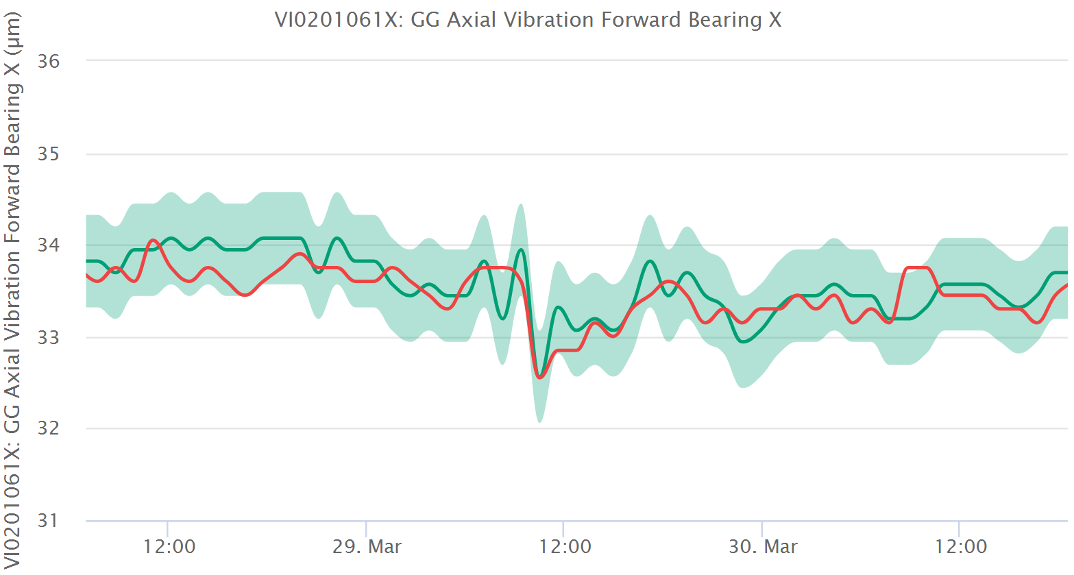
After training, the model is assessed automatically for its goodness and this can be seen in the interface in several different ways. The most direct way is the historical plot of model and measurement in which you can see the time evolution of both the model and the measurement. If they are close during healthy times and far during unhealthy times, the model is doing its job.
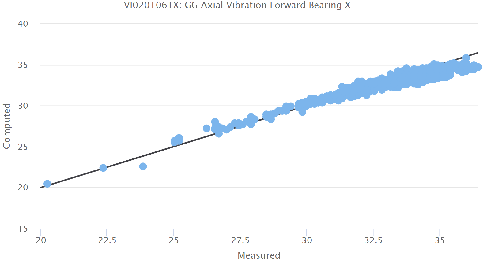
In general we expect the difference between model and measurement to be very small for the training and validation datasets as both are known healthy conditions for the equipment. If we plot the model against the measurement, we would expect to receive a straight line at 45 degrees to both axes. This plot is produced in the interface with a black line drawn at 45 degrees so that we can judge the deviation from the ideal case.
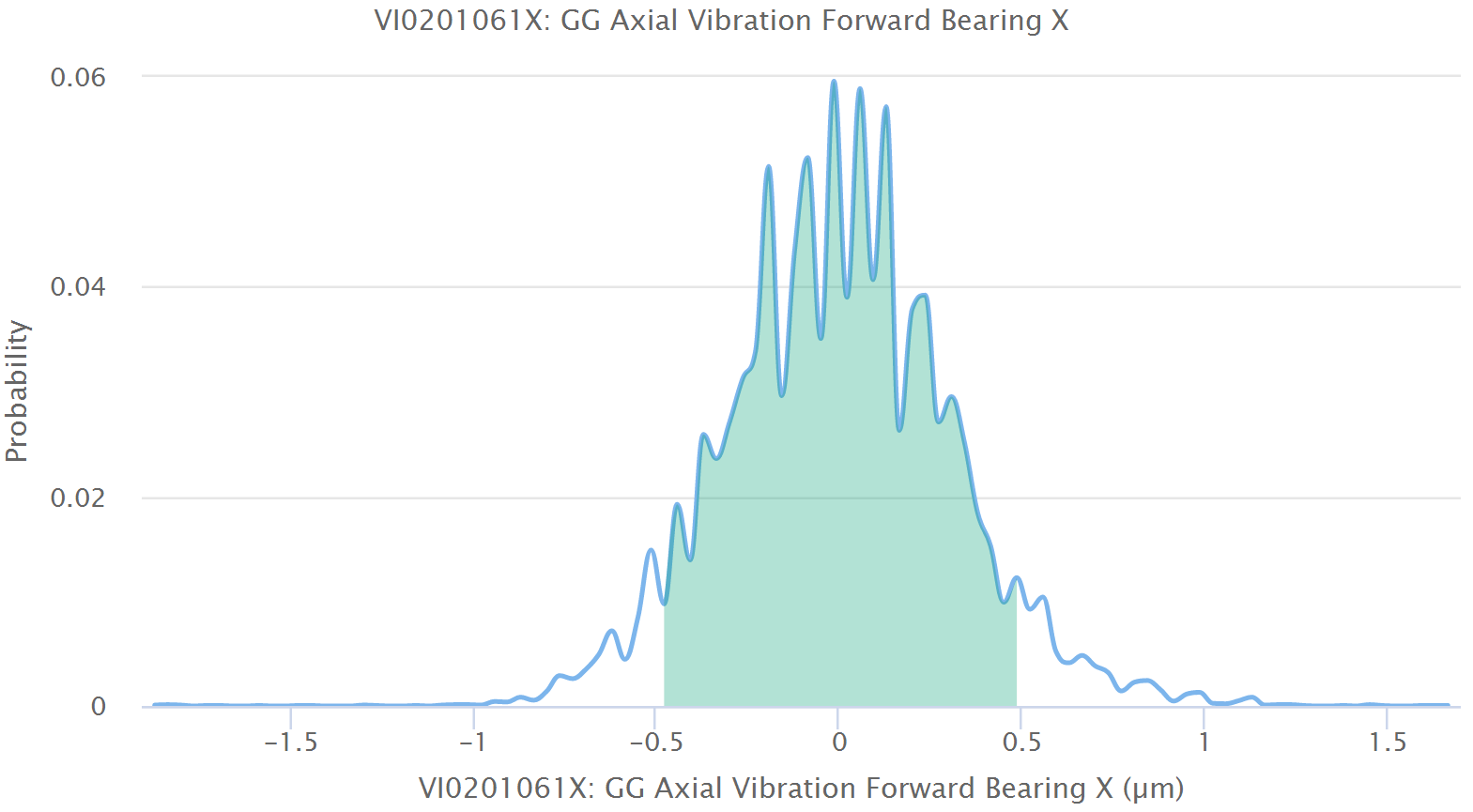
In addition, we expect the deviations between model and measurement to be such that most of them are very small and decreasing amounts are larger and larger. If we plot this deviation on the horizontal axis and the proportion of points that have that deviation on the vertical axis, we receive a probability distribution of the deviations. This is plotted in the interface as well. We would expect this to be a bell-shaped curve, ideally a normal or Gaussian distribution. If that is the case, then this is another indication of good model quality.
We also measure statistical quantities such as mean, standard deviation, skewness and kurtosis for this probability distribution to give further details. In practice a visual inspection of these three diagrams is sufficient to judge if the model is good or not.
If the model is not good, then there are two possible reasons for this. First, the independent variables selected are not the right ones. We must either add some more or remove some disturbing ones. Usually, we have to add variables. Second, the training periods are not long enough or contain unhealthy states. Please check this carefully as the integrity of the data used to define health is the critical element in the entire analysis.
7.1.6. Uncertainty
It is very important to note that all empirical measurements are uncertain. When you step on your bathroom scales in the morning and conclude that you weigh 80kg, ask yourself what this means.
First, the scales have some inherent uncertainty due to the springs being used internally to gauge your weight and turn the readout disc. This measurement uncertainty is usually specified by the manufacturer in the manual.
Second, there is an uncertainty in your reading of the measurement. Since you are looking down at a small disc on the floor, the difference between 80kg and 81kg is barely visible.
Thirdly, there is a change in your condition. Due to the amount of food and drink you consumed in the last hours, your total body weight will change even if you have not gained or lost any fat.
These three sources of error add up to make this measurement uncertain by perhaps about 2kg. So your measurement of 80kg is actually 80 +/- 2kg, i.e. your body weight is somewhere in the range of 78kg to 82kg.
All three of these error sources apply in industrial datasets as well. The sensor has an inherent uncertainty, the measurement chain from sensor to data historian adds a readout uncertainty, and the locally changing conditions at the precise location of the sensor will add variability that is not characteristic of the average situation that one is usually concerned about.
The importance of this lies in the fact that if we use uncertain data in a computation, then the computed result inherits uncertainty from each of its data sources. We can determine the uncertainty in the computed value if we know the measurement uncertainty in the original data. In mathematical modeling, it is as important to have a good model as it is to know how accurate that model is.
7.1.7. Pre-processing
Before raw measurement data can be used in the context of machine learning, it is usually passed through several stages of processing. These methods are collectively called pre-processing and are essential to getting good results.
Implausible values are removed from the dataset according to the allowed ranges of values specified in the metadata. Outliers are removed next. These are data points that exhibit highly irregular or impossible features such as very large gradients. Values that are removed are filled in with the most recent prior plausible measurement.
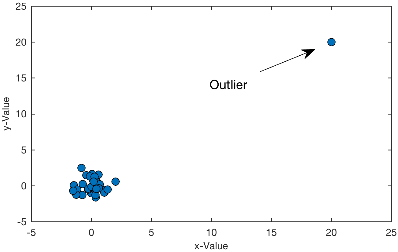
Values are also normalized into a coordinate system so that each variable has an average of zero and standard deviation of one. This removes any natural scaling and thus removes any incompatibility of data related purely to the magnitude of the data. For example, you could measure a weight in kilograms or tons. For human understanding it does not matter much but for a computer the numbers are much larger in kilograms than in tons and so they would receive a different influence in comparison to something else like a pressure. Normalization removes any such features and pays attention only to relative variation in structure.
7.2. Machine Learning
Machine learning, in its basic definition, is a way of representing empirical data in an efficient form, so that it can either be reproduced, generalized, recognized or some pattern in it can be discovered. The goal of machine learning is, then, to summarize data in the form of (a set of) equations.
A very simple example of machine learning would be measuring a series of points that lie on a straight line. The straight line is a model that represents the data we have measured. We use a simple equation to represent the straight line: y, the vertical axis, is equal to m, the slope of that straight line, multiplied by x, the horizontal axis, plus a constant b that is the intercept of the line with the vertical axis. So y = mx + b is a summary of the data and it includes two parameters: m and b. As the measurements for both x and y are imprecise, the model parameters m and b also have uncertainties. This allows the model to cope with the imprecise nature of real life data sets.
Finding the values of m and b from a particular set of empirical data is, as we said, a simple example of machine learning. Thousands of data points have been reduced to two parameters of an equation.
The method of how to compute the parameters of a model from data is called an algorithm. Beyond the algorithm needed to compute the parameters of a model from data, machine learning often needs a second algorithm to update the parameters whenever additional data becomes available. This is not always possible, depending on the model, and represents a serious advantage as initial learning is usually time consuming.
The way a machine approaches learning is not the same as a human, but considering an analogy can be quite useful in the case of neural networks.
The brain is essentially a network of neurons that are connected by synapses. Each neuron and each synapse are individually quite simple objects but in a network they are able to carry out some astonishingly complex actions. Consider putting a name to the face of a person, for example, and connecting that to memories with that person. All this happens unconsciously, within fractions of a second. That's a neural network at work.
As a person is not born knowing all the people they will meet in their life, the brain's neural network gets trained as it experiences things, learns them, and can then draw on this knowledge quickly.
That is similar to how an artificial neural network learns. You start with a prototypical neural network and you start feeding it experiences. The more experiences you show the neural network the more it becomes capable of correctly representing those experiences and recalling them in the future.
The learning of a straight line we discussed is a simple example of machine learning. Neural networks, on the other hand, are capable of representing extremely complex data sets.
7.2.1. Neural Networks
A neural network consists of nodes that are connected to each other (not unlike the neurons, connected by synapses). The input data enters the network on special nodes and then begins to travel through the network. Every time a piece of data travels over a connection or encounters a node, it is modified according to mathematical rules. The modified data then exits the network on other special nodes. Each connection and each node carry parameters that specify exactly what is done there. In this way, the network represents the relationship between the output and the input data and thus represents a mathematical function just like the straight line equation. So a neural network is nothing more than an equation with parameters to be determined from the data that this network is supposed to represent.
All the fuss about neural networks is based on the fact that there exists a mathematical proof which we won't go into here, that shows that if the network has enough nodes in it, then it is capable of accurately and precisely representing any data set, as long as the data set is internally consistent. This holds true even if the relationships in that data set are highly non-linear or time-dependent.
What does internally consistent mean? It means that the source of that data should always obey the same laws. In the case of industrial production, the data is produced by the laws of nature. As they do not change, the data set is internally consistent. The driving forces underlying the stock market, for example, are not constant over time and that is why neural networks cannot represent these data sets well.
In summary, a neural network is a complex mathematical formula that is capable of representing accurately any set of internally consistent data. The general approach to doing this is to take a formula with parameters and to determine the values of the parameters using a computational method. That is what we call machine learning.
It is useful to view a neural network as a summary of data -- a large table of numbers is converted into a function -- similar to the abstract of a scientific paper being a summary. Please note, that a summary cannot contain more information than the original set of data; indeed it contains less! Due to its brevity, however, it is hoped that the summary may be useful. In this way, neural networks can be said to transform information into knowledge, albeit into knowledge that still requires interpretation to yield something practically usable.
The summarization of data is nice but it is not sufficient for most applications. To be practical, we require interpolative and extrapolative qualities of the model. Supposing that the dataset included measurements taken for the independent variable x taking the values x=1 and x=2, then the model has the interpolative quality if the model output at a point in between these two is a reasonable value, i.e. it is close to what would have been measured had this measurement been taken, e.g. at x=1.5. Of course, this can only hold if the original data has been taken with sufficient resolution to cover all effects. The model has the extrapolative quality if the model output for values of the independent variable outside the observed range is also reasonable, e.g. for x=2.5 in this case. If a model behaves well under both interpolation and extrapolation, it is said to generalize well.
A neural network model is generally used as a black-box model. That is, it is not usually taken as a function to be understood by human engineers but rather as a computational tool to save having to do many experiments and determine values by direct observation. It is this application that necessitates both above aspects: We require a function for computation and this is only useful if it can produce reasonable output for values of the independent variables that were not measured (i.e. compute the result of an experiment that was not actually done having confidence that this computed result corresponds to what would have been observed had the experiment been done).
7.2.2. Feed-Forward Networks
Generally, most neural network methods assume that the data points used to train it are independent measurements. This is a pivotal point in modeling and bears some discussion.
Suppose we have a collection of digital images and we classify them into two groups: Those showing human faces and those showing something else. Neural networks can learn the classification into these two groups if the collection is large enough. The images are unrelated to each other; there is no cause-effect relationship between any two images — at least not one relevant to the task of learning to differentiate a human face from other images.
Suppose, however, that we are classifying winter versus summer images of nature and that our images were of the same location and arranged chronologically with relatively high cadence. Now the images are not independent but rather they have a cause-effect relationship ordered in time. This implies that the function f(…) that we were looking for is really quite different. Its accuracy would be a lot better if it did not assess each image on its own merits but rather had a memory of the last few images because often a few images of summer, we are likely to get another image of summer. In this version, we see a dependence upon history that implies a time-oriented memory of the system over a certain time scale that must somehow be determined.
As a consequence of this, we have network models that work well for datasets with independent data points and others that work well for datasets in which the data points are time-dependent. The networks that deal with independent points are called feed-forward networks and form the historical beginning of the field of neural networks as well as the principal methods being used. The networks that deal with time-dependent points are called recurrent networks, which are newer and more complex to apply.
The most popular neural network is called the multi-layer perceptron and takes the form y = aN(WN · aN-1(WN-1 · … a1 (W1 · x + b1) … + bN-1) + bN) where N is the number of layers, the W_i are weight matrices, the b_i are bias vectors, the tanh(…) are activation functions and x are the inputs as before.
The weight matrices and the bias vectors are the place-holders for the model's parameters. The so-called topology of the network refers to the freedom that we have in choosing the size of the matrices and vectors, and also the number of layers N. The only restriction that we have is the problem-inherent size of the input and output vectors. Once the topology is chosen, then the model has a specific number of parameters that reside in these matrices and vectors.
In training such a network, we must first choose the topology of the network and the nature of the activation functions. After that we must determine the value of the parameters inside the weight matrices and bias vectors. The first step is a matter of human choice and involves considerable experience. After decades of research into this topic, the initial topological choices of a neural network are still effectively a black art. There are many results to guide the practitioners of this art in their rituals but these go far beyond the scope of this book. The second step can be accomplished by standard training algorithms that we mentioned before and also will not treat here.
A single-layer perceptron is thus y = tanh(Wx + b) and was one of the first neural networks to be investigated. The single-layer perceptron can represent only linearly separable patterns. It is possible to prove that a two-layer perceptron can approximate virtually any function of interest to any degree of accuracy if only the weight matrices and bias vectors in each layer are chosen large enough.
7.2.3. Recurrent Networks
The basic idea of a recurrent neural network is to make the future dependent upon the past by a similar form of function like the perceptron model. So, for instance, a very simple recurrent model could be x(t+1) = a(W · x(t) + b). Note very carefully three important features of this equation in contrast to the perceptron discussed before: (1) Both input and output are no longer vectors of values but rather vectors of functions that depend on time, (2) there is no separate input and output but rather the input and output are the same entity at two different times and (3) as this is a time-dependent recurrence relation, we need an initial condition for evaluation.
The network we are going to employ uses the concept of a reservoir, which is essentially just a set of nodes that are connected to each other in some way. The connection between nodes is expressed by a weight matrix W that is initialized in some fashion. Generally it is initialized randomly but substantial gain can be got when it is initialized with some structure. At present, it is a black art to determine what structure this should be as it definitely depends upon the problem to be solved. The current state of each node in the reservoir is stored in a vector x(t) that depends on time t.
An input signal is given to the network u(t) that also depends upon time. This is the actual time-series measured in reality that we wish to predict. The input process is governed by an input weight matrix Win that provides the input vector values to any desired neurons in the reservoir. The output of the reservoir is given as a vector y(t). The system state then evolves over time according to x(t+1) = f(W · x(t) + Win · u(t+1) + Wfb · y(t)) where Wfb is a feedback matrix, which is optional for cases in which we want to include the feedback of output back into the system and f(…) is a sigmoidal function, usually tanh(…).
The output y(t) is computed from the extended system state z(t) = [x(t); u(t)] by using y(t) = g(Wout · z(t)) where Wout is an output weight matrix and g(…) is a sigmoidal activation function, e.g. tanh(…).
The input and feedback matrices are part of the problem specification and must therefore be provided by the user. The internal weight matrix is initialized in some way and then remains untouched. If the matrix W satisfies some complex conditions, then the network has the echo state property, which means that the prediction is eventually independent of the initial condition. This is crucial in that it does not matter at which time we begin modeling. Such networks are theoretically capable of representing any function (with some technical conditions) arbitrarily well if correctly set up.
7.2.4. Clustering
Quantitative data often can be divided into qualitative groups. Operating a gas turbine, for example, we may run it in idle, half load or full load mode. These concepts mean something to a human engineer who understands them. They can be defined for the computer using strict rules based on measurements such as the rotation rate. However, creating such rules brings several problems with it: (1) The rules will necessarily have to be strict and simplistic, (2) a human engineer has to take the time to define them, (3) the rules must be maintained in some system and periodically checked for accuracy as the equipment or plant gets modified over its lifetime, (4) data entry is error prone if we consider the volume of such definitions that are necessary for an industrial plant operating hundreds of such pieces of equipment with hundreds or thousands of measurements each.
All these issues can be resolved if we group operational points together based on data analysis rather than rules generated from human understanding. The attempt to do this is called clustering. In it, we try to determine the number of clusters and their membership over a historical collection of observations subject to two conditions: (1) There should be little variability between the members of any one cluster and (2) there should be a lot of variability between members of two different clusters.
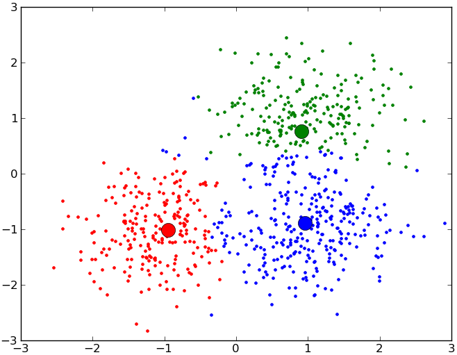
When we deal with quantitative data, we can define a cluster to essentially be a sphere. That is to say a cluster is a point in space with a certain radius. Every historical observation inside this sphere belongs to this cluster and every point outside does not. Clearly, this approach will have to deal with overlapping spheres and with some points that do not fit into any sphere. Nonetheless, this idea is the most popular in clustering.
In practice we thus ask ourselves how many spheres we need, where they are and how big they are in order to satisfy our two criteria. There are methods to do this and will result in a good clustering of any dataset. Unfortunately, these methods are expensive in terms of computation time but they can realistically be applied to industrial grade data.
The benefit of these methods is that they allow an automated event framework to be defined. As the equipment performs its function, we can then easily tell in which condition or event the equipment currently operates. Each time that the equipment changes its condition or event, this fact can be recorded. Both of these features combined can be used to drive a calculator for equivalent operating hours for the equipment as transitioning from one state to another may be quick in clock time but consume far more in terms of equipment lifetime.
7.2.5. Variable Reduction
Much of the data that is stored in a typical data historian in an industrial plant is not needed in order to make reliable statements about equipment health or process optimization. Usually less than 10% of all measurements are actually needed. Of these, there is generally substantial duplication of information in the data.
Whenever we want to model a system, the first task is to intelligently select the necessary data. There is a danger in giving the analysis not enough data and so we usually err on the side of caution and include a number of measurements of which we are not sure whether they add information or not. To avoid unnecessarily cluttering the analysis with superfluous data, we must determine which measurements are actually important and which are not.
On top of that, some measurements are correlated with each other and so add some information but not as much as others. Take for example your own body weight, height, sex and level of physical activity. Based on your height, sex, and level of physical activity one cannot know your weight but one can make a reasonable statistical guess at your weight. Measuring your weight after this estimation provides additional information but not as much as the original three values provided because your weight is correlated with them. Depending on what one wishes to figure out about a person, one may be able to do it without knowing this additional piece of information and make do with the original ones.
Based on these insights, we get two different ideas for reducing the number of variables in a model. We could identify variables that are not needed at all and simply exclude them from the model altogether. Secondly, we may transform the dataset into a different coordinate system with fewer dimensions in which, however, each of the new dimensions is a combination of the original dimensions. This second idea is based on the insight described above that some measurements provide a little extra information and should thus not be thrown out altogether but are not really worth a full dimension.
This idea leads to principal component analysis, which is best explained visually.
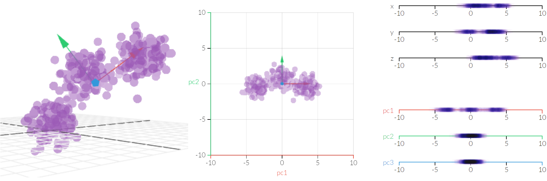
The selection of how many principal components are needed to explain the information in a dataset can be made precise using statistical information. In this case, it was clear to a human viewer that one dimension is enough to separate the three classes of data points. If we are dealing with reducing 10,000 dimensions to 500, then this will no longer be visible to a human user but can nevertheless be made precise.
We use this method to reduce the dimensionality of the dataset while maintaining the amount of information contained in it. The ultimate benefit is that we can model the dataset using significantly less parameters without sacrificing (much) accuracy. This not only saves time but also improves the generality of the model as it is a general truth in machine learning that a model with fewer parameters has greater power of generalization to data that was not learned.
7.3. Optimization
There are many optimization approaches. Most are exact algorithms that definitely compute the true global optimum for their input. Unfortunately such methods are usually intended for a very specific problem only. There exists only one general strategy that always finds the global optimum. This method is called enumeration and consists of listing all options and choosing the best one. This method is not realistic as in most problems the number of options is so large that they cannot be practically listed.
All other general optimization methods derive from enumeration and attempt to either exclude bad options without examining them or only examine options that have a good potential based on some criteria. Particularly two methods, genetic algorithms and simulated annealing, have been successful in a variety of applications. The later advent of genetic algorithms stole the limelight from simulated annealing for some time. However, from direct comparisons between these two approaches it appears that simulated annealing nearly always wins in all three important categories: implementation time, use of computing resources (memory and time) and solution quality. Thus, we shall focus on simulated annealing.
7.3.1. Simulated Annealing
When an alloy is made from various metals, these are all heated beyond their melting points, stirred and then allowed to cool according to a carefully structured timetable. If the system is allowed to cool too quickly or is not sufficiently melted initially, local defects arise in the system and the alloy is unusable because it is too brittle or displays other defects. Simulated annealing is an optimization algorithm based on the same principle. It starts from a random point. This is modified by moving to a nearby point. The new point is compared with the old one. If it is better, we keep it. If it is worse, we keep it with a certain probability that depends on a "temperature" parameter. As the temperature is lowered, the probability of accepting a change for the worse decreases and so uphill transitions are accepted increasingly rarely. Eventually the solution is so good that improvements are very rare and accepted changes for the worse are also rare because the temperature is very low and so the method finishes and is said to converge. The exact spelling out of the temperature values and other parameters is called the cooling schedule. Many different cooling schedules have been proposed in the literature but these have effect only on the details and not the overall philosophy of the method.
We immediately see some rather enticing features: (1) Only two solutions must be kept in memory at any one time, (2) we must only be able to compare them against each other, (3) we allow temporary worsening of the solution, (4) the more time we give the algorithm, the better the solution gets and (5) this method is very general and can be applied to virtually any problem as it needs to know nothing about the problem as such. The only points at which the problem enters this method is via moving the point and via comparing two points.
8. Terminology
In this chapter, we offer definitions of some of the terms that occur frequently in the interface. These terms have received shorter descriptions elsewhere in the manual and interface and are treated with greater detail here.
8.1. Plant
The plant is that entire entity that is being modeled. It does not necessarily need to be identical with the entirety of a particular organizational or corporate unit. For example, a power plant may decide to model only the turbine. Conversely, a chemical plant may decide to include data from up and down stream into its model thereby enlargening it beyond the corporate unit.
To distinguish one plant from another, we offer four database fields with which to name the plant: Company, division, plant and equipment. An example for these would be XY Corporation, Chemical Division, Sampletown, Turbine.
8.2. Tag
A sensor is a physical device that converts some aspect of a physical situation into a numerical value relative to some agreed-upon scale. A temperature sensor, for example, will output the temperature of its ambient medium as a numerical value on the Celcius or Fahrenheit scale.
It is important to note that sensors suffer from several sources of error that must be taken into account when interpreting the numerical value in question.
First, each sensor has a measurement uncertainty, specified by its manufacturer, that illustrates that the same physical situation may lead to results anywhere within a numerical range of this size.
Second, every sensor suffers from drift over time. With age, accumulation of dirt and other factors, the numerical output value has a tendency to steadily rise or fall. This leads to the need to periodically calibrate sensors or replace them.
Third, a sensor may have a systematic error due to its placement. For example, a temperature sensor placed on the outside of a large vessel will measure the temperature there but this temperature will not be equal to the average temperature in the vessel. For machine learning analysis, this effect usually does not influence model quality as the error is always constant. However, this error is significant if a physical interpretation is needed. For example, if we know that the best temperature is 100 degrees and we measure 98 degrees, we may be tempted to inject heat but this may not be necessary as the outside of the vessel may legitimately be 2 degrees cooler than its average internal temperature.
A measurement is an individual numerical result delivered by a particular sensor. A measurement is thus always three pieces of information: The time at which it was taken, the tag it is relevant to, and the value that was recorded.
A tag encapsulates a regular measurement made by a sensor and all the data associated to that operation. If the sensor must be exchanged or recalibrated, the tag remains the same. All the data ever recorded relative to that quantity is stored under the tag's identification. Tags are therefore the currency on which all process models are built.
A sibling to a tag is another tag that measures the same quantity in the same manner in roughly the same location. We desire to have siblings in the case of important measurements for which we cannot afford a sensor malfunction or failure. A normal industry standard is to install three sensors and, at any one time, use the average of the two measurements that most closely agree as the true value measured by the triplet of sensors. In case the siblings disagree significantly with each other, we have two potential problems. Either a sensor is malfunctioning or the equipment truly exhibits this deviation in between the (usually very close by) locations of the sensors in which case the equipment is probably in an unhealthy state.
8.3. Minimum and Maximum
The normal range of values is defined by providing each tag with a minimum and maximum value. These two values define the range of numerical values that this tag can reasonably have. If a tag’s value at some time in history does not lie in this range, the entire operational point of the plant at this time will be excluded from the training data set.
Let’s take an example. A chemical process requires a temperature of 250°C. In the actual process, the temperature will actually vary between 220 and 270°C. A temperature above 270°C will trigger an automatic shutdown. However if the plant is offline, the temperature will slowly adjust to the ambient temperature, which may be as low as -20°C. Thus, the range should be -20°C to 270°C because the plant being offline is a valid state.
Let’s take a second example. A valve can be opened and closed. Its status is measured in percent. Strictly speaking therefore, the range is 0 to 100% from fully closed to fully open. However, the sensor that measures the status sometimes measures values slightly lower than 0 or slightly higher than 100. We can approach this problem in two ways. Either we can define the range to lie between -5% and 105% or we can define the range to lie between 0 and 100% and additionally define two correction rules that will force any measurement below 0 to be equal to 0 and any measurement above 100 to be equal to 100.
After you have set the metadata for the plant, the analysis will perform a plausibility check. Among other things, this check will compute how many historical operational points of the plant will be ignored based on the range setting of each tag. You can use this information to adjust your settings. In addition, each tag has its own properties page that contains a histogram displaying the distribution of its values. You may use this to gain insight into what values a tag actually adopts much of the time.
Frequently we find that some ranges are defined such that all, or very close to all, operational points become disallowed for modeling. This is usually the case because the range is a theoretically desired range that is not actually obeyed in real operations or because of various errors, for example that the tag is actually measured in different units than expected. If the tag is in tons and the range is set in kilograms, then this will happen.
8.4. Static Alarm Limits
In addition to the dynamic limits computed by IHM, normal static limits are supported by IHM. The green area should enclose normal operational values, yellow the dangerous ones, orange the critical ones and red the failure ones. You may use any or all of these colored areas as you choose. Through IHM you will then be alarmed when the measurement value crosses any defined limit value towards a worse state. The colored regions can be defined for each tag by specifying the boundaries between the colored regions. Please see the images below for an illustration.
8.5. Controlability
The controllability of a tag is one of three possibilities. A tag is either controllable, uncontrollable or semi-controllable. Choosing which of these categories any one tag falls into is probably the most important choice you will make regarding the mathematical modeling of your plant.
A tag is controllable if it can be modified manually by the operator of the plant. For that, it is usually a set point value. In a plant, there might be quite a few PID controllers in operation that automatically control various values based on others. While an operator might have the theoretical capability of turning a PID controller off and taking that controlled value into manual operation, chances are that this is not desired and rarely done. Thus, this value is only theoretically controllable but not actually controllable. We should mark as controllable only those values that are actually modified by the operators of the plant. It may be a good idea to have a conversation with an operator in the control room to come up with a list of tags that are actually available for direct modification.
Only those tags should be marked as controllable that could possibly have an impact upon the performance aspect of the plant that you wish to optimize. For example, there will be a few tags that have relevance for emergency procedures or start ups and shut downs that are actually manually controlled. But we are not interested in modifying these in order to optimize normal performance.
Every controllable tag is allowed to appear in a suggestion to the operator to change the plant’s state. At any one time, it may not be necessary to change the value of every controllable tag but usually every controllable tag appears in some suggestions. You can see how often each tag appears in a suggestion in the report that you can read after the modeling step.
A tag is uncontrollable if it cannot be modified in any way by the operator of the plant. These are tags that measure the status of the outside world. Aspects of the weather such as temperature, humidity, and air pressure are examples. The quality of raw materials is usually an important aspect. Usually the amount of product that a plant produces is a major limiting amount that is prescribed by the customers of the plant.
Clearly there are many things that an operator cannot control. However, we should only include those aspects of the outside world that actually have an influence on the performance of the plant. If you believe the outside air temperature to influence the process (it usually does), then include it. There are some processes that are sensitive to humidity but most are not. While you probably measure humidity in your local weather station, only include it in the model as uncontrollable if you believe it to have an effect.
An uncontrollable tag is a boundary condition for the plant. The mathematical model that will be constructed will look for an operational point that is better than the current point but that has the same values for all uncontrollable tags. Every uncontrollable tag restricts the freedom of the optimizer and thereby reduces the possible improvement that the optimizer can achieve. Thus choosing which tags are uncontrollable has an important effect on the model.
Every tag that is neither controllable nor uncontrollable is therefore semi-controllable. These are all the tags that cannot be directly modified but are indirectly modified through the controllable tags. The large majority of available tags will be in this category and this is considered the default setting. When creating your list of tags, we strongly suggest that you start by regarding every tag as semi-controllable and then continue by marking those tags as controllable or uncontrollable that you identify as being so. In this way, you will end up with a list of relatively few and carefully chosen tags that can and should be modified and tags that represent restrictions to the plant.
8.6. Correlation
When two different tags have a relationship, they are called correlated. When we speak of correlation, we typically mean that the relationship is linear. This means that when one tag varies, the other tag varies proportionally to the first, i.e. the relationship is expressed by the constant of proportionality.
An example of two correlated tags is the temperature and pressure of a substance in a vessel. As long as the vessel retains its volume and no substance is allowed to enter or leave the vessel, the pressure and temperature are directly related to each other; as one increases, so does the other. These two tags are strongly related in this fashion and so they are highly correlated.
Another example of two correlated tags is the rotation rate and vibration amplitude. However this relationship depends on a multitude of other tags as well. While these two will tend to increase and decrease together, one might vary somewhat without the other due to other conditions. This relationship is thus weaker.
The strength of a correlation is measured by the correlation coefficient that is a number between -1 and 1. If the coefficient is 1, then the two tags will vary in exact mutual relationship. If the coefficient is -1, the same is true except that while one tag increases, the other decreases. If the coefficient is somewhere in the middle, the relationship is weaker. In real-life data, no two tags are ever correlated perfectly as there is always a natural random variation in any measurement; at the very least due to measurement uncertainty.
In general, it is not possible to interpret a single correlation coefficient in a precise manner because correlation depends on context. For example, if two tags are correlated with a coefficient of 0.758, what does this mean? By itself, this does not mean much. In comparison, correlation coefficients acquire meaning. If two tags have a coefficient of 0.758 and two others have a coefficient of 0.123, then we can say that the first pair is much more related than the second pair. What correlation coefficients are called high or low is a subjective decision of the observer.
In industrial data sets, we sometimes observe correlation coefficients above 0.95 between related tags and frequently get coefficients above 0.8.
We can compute a correlation matrix for a collection of tags in which we compute the correlation coefficient between every pair of tags. This matrix can then be analyzed to ask: What tags are most related to a particular tag? We could choose the tags that are most highly correlated to the tag of interest. We may, additionally, look at the correlation between the tags selected and throw out any tags that have high mutual correlation because this would indicate a (near) duplication of information.
The correlation matrix can form the basis for putting the tags into clusters. Generally, highly correlated tags are physically connected and thus would belong to a single cluster.
8.7. Sensitivity
The concept of sensitivity is closely related to that of correlation in that we ask how closely two tags are related. Correlation is usually used in the context of a linear relationship whereas sensitivity is usually used in a general, i.e. linear or non-linear, context. Particularly, sensitivity is used in the context of a mathematical model.
If we have a formula such as y = f(a, b), then we might ask: How much will y vary as a or b vary? If it turns out that y varies a lot as a varies but not very much at all as b varies, then we might think that we could simplify the formula by excluding b from the formula.
Sensitivity thus plays an important role in an attempt to simplify models or to reduce the number of variables in a model. It also plays an important role in gauging how much influence one might have over y. If, for example all the tags that have a high sensitivity with y cannot be controlled, then it will be difficult to exert control over y. In this case y is dominated by its environment. If, on the other hand, one or more tags that have high sensitivity can be controlled, then it may be possible to use the model for advanced process control.
The models built in IHM and ISS indicate the sensitivities of the independent variables and thus provide some insight to the user either in an effort to simplify the model or to decide how useful the model is.